Classification Metrics

Authors:

Published On:

Aug 6, 2026

Last Updated:

Aug 9, 2026

Once you have trained a classifier, you need some way of describing how good it is. The obvious first attempt is accuracy, which is the percentage of predictions that were correct. But on its own this is a poor measure, and on some problems it is actively misleading! Precision and recall split that single number into two, and between them they describe the two different ways a classifier can be wrong.

The Confusion Matrix

The confusion matrix (aka error matrix) is a table that compares the predictions of a classifier against the true labels. It breaks down the predictions into four categories:

True positive (TP): predicted positive, and it really was positive.
False positive (FP): predicted positive, but it was actually negative. Also called a type I error, or a false alarm.
False negative (FN): predicted negative, but it was actually positive. Also called a type II error, or a miss.
True negative (TN): predicted negative, and it really was negative.

Arranged into a grid, these form the confusion matrix:

The confusion matrix.

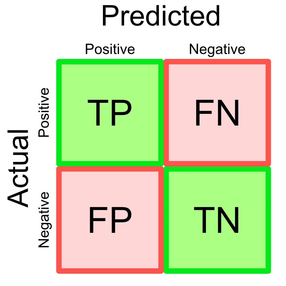
The whole confusion matrix is worth looking at directly. Collapsing it into a single number always throws information away, and which information you can afford to lose depends entirely on the problem.

Accuracy

Accuracy is the fraction of all predictions that were correct:

\text{accuracy} = \frac{\text{TP} + \text{TN}}{\text{TP} + \text{TN} + \text{FP} + \text{FN}}

This is fine when the classes are roughly balanced, and badly broken when they are not. Suppose you are inspecting PCBs coming off a production line, and 1 in 100 has a defect. A “classifier” consisting of the single line return NOT_DEFECTIVE; scores 99% accuracy whilst being completely useless — it never finds a single defect. Worse, it will beat a genuinely useful model that catches most defects at the cost of a few false alarms.

This is the key problem with accuracy: it lets the majority class dominate the score. Since the interesting class is usually the rare one (defects, faults, disease, fraud), accuracy tends to be least trustworthy exactly when you care most.

Precision

Precision asks: of everything the classifier flagged as positive, what fraction really was positive?

\text{precision} = \frac{\text{TP}}{\text{TP} + \text{FP}}

The denominator is everything the classifier said “yes” to. Precision is therefore about the cost of false alarms. A low precision means you are crying wolf, and whoever (or whatever) acts on the classifier’s output will waste effort chasing things that turn out to be nothing. In situations in where false alarms are expensive, you want a high precision.

Recall

Recall asks the complementary question: of everything that really was positive, what fraction did the classifier find?

\text{recall} = \frac{\text{TP}}{\text{TP} + \text{FN}}

Here the denominator is everything that was actually positive, whether the classifier spotted it or not. Recall is about the cost of misses. A low recall means real cases are slipping through undetected.

Recall goes by several other names: sensitivity, the true positive rate, and (in a detection context) the probability of detection.

The Trade-off Between Them

Precision and recall trade off with one another. Most classifiers do not output a hard yes/no and instead internally produce a score or probability. A chosen threshold then turns that into a detection. Moving that threshold trades precision for recall:

Raise the threshold (only say “positive” when very confident): fewer false positives, so precision rises. But you also miss borderline true cases, so recall falls.
Lower the threshold (say “positive” on the slightest suspicion): you catch more real cases, so recall rises. But you also flag more things that turn out to be negative, so precision falls.

The two extremes make this obvious. Flag everything as positive and recall is a perfect 1.0, whilst precision collapses to the base rate of the positive class. Flag nothing and precision is vacuously perfect (or undefined) whilst recall is 0.

This is why quoting one of them alone is meaningless — “our detector achieves 99% recall” says nothing if it flags half the dataset to get there. Always quote precision and recall together.

Which one you should favour is not a modelling question, it is a question about the application:

Favour recall when a miss is expensive. Screening for a serious disease, detecting a gas leak, or finding safety-critical faults — a false alarm costs you a follow-up check, whereas a miss can be catastrophic.
Favour precision when a false alarm is expensive. An alarm that wakes someone at 3am, a spam filter deleting real email, or any automated action that is hard to undo. Here the cost of being wrong when you act outweighs the cost of occasionally doing nothing.

The F1 Score

Sometimes you do need one number — to rank models, or to drive an automated hyperparameter search. The F1 score combines precision and recall by taking their harmonic mean:

F_1 = \frac{2}{\frac{1}{\text{precision}} + \frac{1}{\text{recall}}} = 2 \cdot \frac{\text{precision} \cdot \text{recall}}{\text{precision} + \text{recall}}

It varies between 0 and 1, with 1 being perfect.

The reason for using the harmonic mean rather than the ordinary arithmetic mean is that the harmonic mean is dominated by the smaller of the two values, so it punishes a classifier that is lopsided. Consider the “flag everything as positive” classifier from earlier applied to those PCBs, with a precision of 0.01 and a recall of 1.0:

Arithmetic mean: $\frac{0.01 + 1.0}{2} = 0.505$ . Classifier is genuinely worthless, but gets an ok score (not great, but not horrible!)
Harmonic mean: $\frac{2 \cdot 0.01 \cdot 1.0}{0.01 + 1.0} = 0.0198$ . The harmonic mean shows the true awfulness of the classifier (lower number drags down the total).

To score well on F1 you have to be good at both, which is exactly the property you want from a summary metric.

If you have done any circuit design, this might seem familiar! The $F_1$ equation is the same (almost) as the one used for two resistors in parallel:

R_{parallel} = \cfrac{1}{\frac{1}{R_1} + \frac{1}{R_2}} = \frac{R_1 R_2}{R_1 + R_2}

The only difference is the numerator. The harmonic mean has an $n$ (here 2, the number of values) where the parallel resistance has a 1, so $F_1 = 2 R_{parallel}$ . That factor is what makes the harmonic mean a mean: without it, “averaging” two equal values of $R$ would give you $R/2$ rather than $R$ .

The behaviour is identical though. A parallel resistor combination is always dragged down towards the smaller resistor, e.g. 1Ω in parallel with 1MΩ gives you very nearly 1Ω, and the big resistor barely matters. That is precisely why $F_1$ refuses to be impressed by a recall of 1.0 when the precision is 0.01.

Note that F1 weights precision and recall equally, which may not be what you want (perhaps the cost of false positives is much more significant?). The more general $F_\beta$ score lets you weight one over the other, with $\beta > 1$ favouring recall and $\beta < 1$ favouring precision:

F_\beta = (1 + \beta^2) \cdot \frac{\text{precision} \cdot \text{recall}}{\beta^2 \cdot \text{precision} + \text{recall}}

$F_2$ and $F_{0.5}$ are the common choices.

A defect detector is run over 10,000 PCBs, of which 100 are genuinely defective. The model flags 80 boards as defective, and on inspection 60 of those really are.

That gives us the four counts:

$\text{TP} = 60$ (flagged and defective)
$\text{FP} = 80 - 60 = 20$ (flagged but fine)
$\text{FN} = 100 - 60 = 40$ (defective but missed)
$\text{TN} = 10000 - 60 - 20 - 40 = 9880$ (not flagged and fine)

The accuracy is:

\text{accuracy} = \frac{60 + 9880}{10000} = 0.994

99.4% — which sounds excellent, and is barely better than the do-nothing classifier’s 99%. Now the two useful metrics:

\text{precision} = \frac{60}{60 + 20} = \frac{60}{80} = 0.75

\text{recall} = \frac{60}{60 + 40} = \frac{60}{100} = 0.60

So from the boards that came off the line, 75% really were faulty (25% of the operator’s inspection time is wasted), and we are catching only 60% of the defects — 40 bad boards per batch are still shipping. The F1 score is:

F_1 = 2 \cdot \frac{0.75 \cdot 0.60}{0.75 + 0.60} = \frac{0.9}{1.35} = 0.667

Notice how far apart 0.994 and 0.667 are. Both are “correct” in their own right; the accuracy figure is just measuring something you do not care about, because it is dominated by the 9,880 good boards the model trivially got right.

Confusion Matrix Calculator

The calculator below calculates various classification metrics from the four confusion matrix counts (TP, FP, FN, TN). It starts pre-seeded with the PCB example from above.

If instead of the confusion matrix counts you have counts of how many samples there were, how many were actually positive, how many the model flagged and how many of those flags were right — switch to Enter scenario and enter the data in that form.

Enter the four confusion-matrix counts (or describe the scenario) to get every metric on this page computed at once. Defaults are the PCB-defect example from above.

Enter countsEnter scenario

Predicted positive

Predicted negative

Actually positive

Actually negative

Prevalence(TP+FN) / N

1.00 %

SamplesN

10,000

Accuracy(TP+TN) / N

0.9940

Classes are imbalanced (prevalence 1.00 %), so accuracy is dominated by the majority class. This score is only 0.0040 better than a classifier that always guesses "negative". Read precision and recall instead.

↳ baselinealways guess "negative"

0.9900

Balanced accuracy(TPR + TNR) / 2

0.7990

MCCMatthews correlation

0.6679

PrecisionPPV — TP / (TP+FP)

0.7500

NPVTN / (TN+FN)

0.9960

RecallTPR — TP / (TP+FN)

0.6000

SpecificityTNR — TN / (TN+FP)

0.9980

FPR1 − specificity

0.0020

FNR1 − recall

0.4000

F₁harmonic mean of P and R

0.6667

F_ββ = 1.0

0.6667

If the classes are imbalanced (e.g. the number of true positives is much smaller than the number of true negatives), the accuracy statistic shows a warning highlighting that it is not a good measure of performance.

More Than Two Classes

Precision and recall are defined for a binary problem, so for a multi-class classifier they are calculated per class — treating that class as “positive” and every other class as “negative” — giving you one precision and one recall for each class. This is what scikit-learn’s classification_report prints: a row per class, plus a support column, which is simply how many instances of that class were actually present in the test data.

To reduce those per-class figures to one number, they get averaged, and there are three ways of doing it that you will see quoted:

Macro average: the unweighted mean across classes. Every class counts the same regardless of how rare it is, so a poorly-handled rare class drags the score down.
Weighted average: the mean weighted by each class’s support. Common classes dominate, which reintroduces the imbalance problem accuracy has.
Micro average: pool the TP/FP/FN counts across all classes first, then compute the metric once. For single-label multi-class problems this ends up equal to accuracy.

Macro is usually the honest choice when the rare classes are the ones that matter.