Sallen-Key Filters

The Sallen-Key filter is one of the most popular active 2nd-order analogue filter topologies.1 It can be configured as a low-pass, high-pass, band-pass or band-stop filter. Also called a Sallen and Key filter. It was first introduced in 1955 by R.P. Sallen and E.L. Key of MIT’s Lincoln Labs, whose last names give this filter its name. It is a filter topology, and defines the components and connections between them to realize a 2nd order filter. Various filter tunings such as Butterworth, Bessel and Chebyshev can be implemented using the Sallen-Key topology.
The Sallen-Key filter has low component spread (low ratios of highest to lowest capacitor and resistor values). It also has a high input impedance and low output impedance, allowing for multiple filters to be chained together without intermediary buffers.
The performance of a Sallen-Key filter does not depend that much on the performance of the op-amp. This is because the op-amp is used as an amplifier, rather than an integrator, which minimizes the gain-bandwidth requirements of the op-amp.1 However there are high-frequency limitations to the Sallen-Key filter, which are explained in more detail below.
One disadvantage of the Sallen-Key filter is that the Q of the filter is very sensitive to component variations, which can be a problem, especially for high-Q filter sections.
The Sallen-Key filter is closely related to a voltage-controlled voltage source (VCVS) filter. Some literature makes the distinction of a Sallen-Key filter having unity gain, and the VCVS filter including non-unity gain by connecting a resistor divider from the output to the inverting terminal of the op-amp. However we will consider them one and the same for the purpose of analysis, as the unity-gain version is a special subtype of the generalized variable-gain version.
Another popular alternative to the Sallen-Key topology is the Multiple Feedback (MFB) topology.2
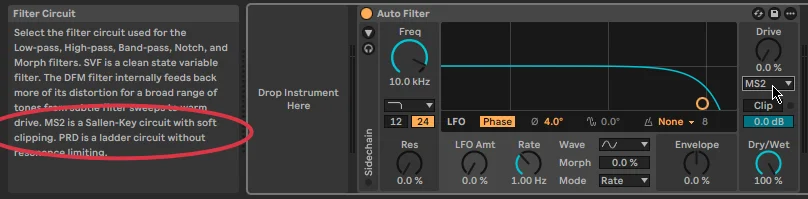
I do a bit of music production, I was interested to find that the Ableton Live Auto Filter has an option called MS2 which is based on the Sallen-Key topology (it is modelled on the filters used in a famous semi-modular Japanese monosynth3). This is a placeholder for the reference: fig-ms2-sallen-key-filter-in-ableton shows a screenshot of the filter in Ableton.
Low-Pass Sallen-Key Filter
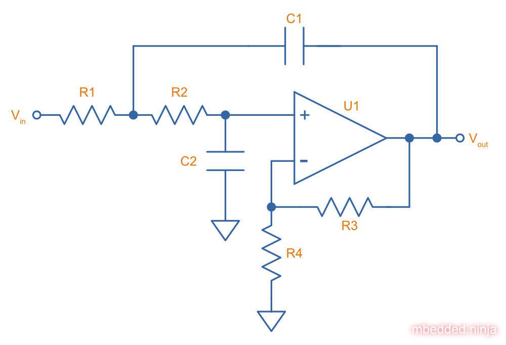
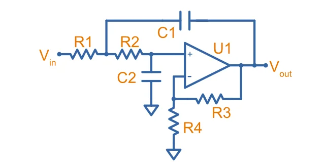
This is a placeholder for the reference: fig-low-pass-variable-gain-sallen-key-filter-schematic shows the schematic for a variable-gain low-pass Sallen-Key filter (a.k.a. VCVS filter).
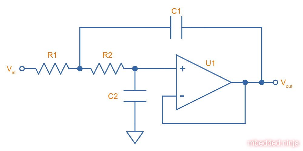
This is a placeholder for the reference: fig-low-pass-unity-gain-sallen-key-filter-schematic shows the schematic for the unity-gain low-pass Sallen-Key filter (which is generally not called a VCVS filter). Note the removal of and , the output is instead directly fed into the inverting input of the op-amp, just like when using an op-amp as a buffer. The filter has unity gain in the pass-band.
The generalized transfer function for a 2nd-order low-pass filter is1 4:
where:
is the gain factor
is the characteristic frequency in radians/s []
is the quality factor and is dimensionless []
Written in the same form as the general equation above, the transfer function for a 2nd-order low-pass Sallen-Key filter is1:
Equating the coefficients in the general form () with those specific to the Sallen-Key topology () allows us to find the equations of the characteristic frequency and quality factor.
The cut-off frequency is (remembering ):
and the quality factor is:
The gain equation is the same as for a non-inverting amplifier:
How To Calculate Component Values
Setting Filter Components As Ratios
The idea here is to define a new variable which is the ratio of the resistances and a new variable which is a ratio of the capacitances.
So we define:
This simplifies the cut-off frequency and quality factor equations to:
Firstly, you decide on a desired gain and quality factor . Then chose a ratio for the capacitors, for example . This will allow you to calculate using the equation for the quality factor.
With arbitrary , and , solving the quality factor equation for gives something truly horrible (I cheated and got Wolfram Alpha to solve this one for me):
Lastly, decide on your cut-off frequency and then you can calculate using the cut-off frequency equation.
The process can be simplified even more, by setting . This makes both capacitors equal.
Tuning Based Design
You can design a Sallen-Key filter based on a particular filter tuning and its coefficients, this is an alternative to choosing the quality factor and gain yourself. Given the filter tuning coefficients and and desired cut-off frequency you can then calculate the required resistances and capacitances.
The resistance of the resistors and are related to the capacitances and filter coefficients by the following equation:
You use the sign when calculating and the sign for calculating .
To obtain real values under the square root, must obey the follow condition:
These equations give you enough info to calculate all the resistances and capacitors for a Sallen-Key filter. See the design example below to show how you would go about it.
Frequency Limitations of the Low-Pass Sallen-Key Filter
A low-pass Sallen-Key filter is strongly dependent on the op-amp having a low output impedance. An op-amp’s output impedance increases with increasing frequency, thus the performance of the Sallen-Key low-pass begins to suffer at high frequencies. This typically manifests itself with the -40dB/decade gain turning around and beginning to increase again after a certain frequency in the stop band of the filter.
This phenomenon can be best understood by analyzing the behaviour at high frequencies. At frequencies much higher than the cut-off frequency , we can treat the capacitors as shorts. This gives rise to the equivalent circuit in This is a placeholder for the reference: fig-low-pass-variable-gain-sallen-key-filter-freq-limit. Shorting means that the op-amp’s non-inverting input is kept at ground (for high frequency signals), and so nothing should pass from input to output. This is true as long as the op-amp has strong enough “drive” to keep this basic tenet true. Unfortunately, as frequency increases, so does the op-amp’s output impedance. This impedance affects the op-amp’s ability to keep the output at , and the gain begins to rise again.
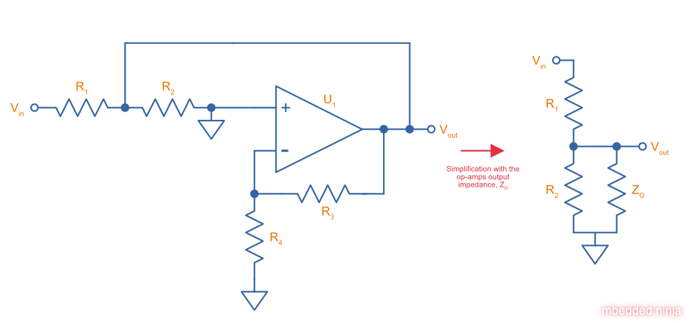
Based on the above schematic, we can use the voltage divider rule to write out the transfer function as:
Assuming is much smaller than , and that and are roughly in the same order of magnitude, the term then dominates the bottom of the fraction. Thus:
is the closed-loop impedance. It is frequency-dependent, and is related to the open-loop impedance by:
where:
is the open-loop impedance
is the open-loop gain
is the feedback factor, and equal to
So as the open-loop gain of the op-amp begins to drop at high frequencies, the output impedance of the op-amp begins to increase. The op-amp then struggles to keep the inverting input of the low-pass Sallen-Key filter at virtual ground, and begins to let through some of the signal. This reduces the effectiveness of the low-pass filter in the stop band.
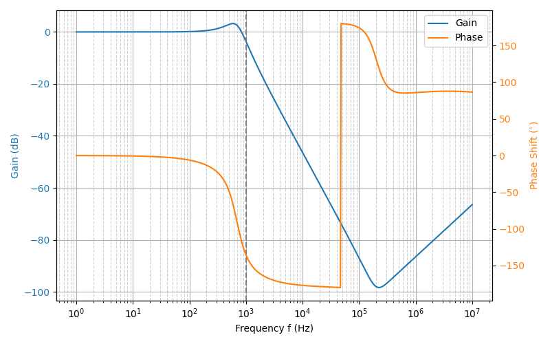
We can see the effect of an increasing output impedance at high frequencies in bode plot of This is a placeholder for the reference: fig-low-pass-sallen-key-showing-gain-rise-annotated-plot for a 2nd-order low-pass Sallen-Key filter, with a cutoff frequency of 1kHz.

High-Pass Sallen-Key Filter
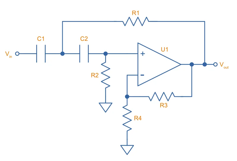
You can arrive at a high-pass Sallen-Key filter by switching the positions of the resistors and capacitors in a low-pass Sallen-Key filter (just like you can for passive RC filters). This gives you the schematic below:
The general form of the transfer function for a second order high-pass filter is1:
Using Ohm’s law and Kirchhoff’s current/voltage laws, we can write the equivalent transfer function for a variable-gain high-pass Sallen-Key filter, in terms of the resistances and capacitances1:
If you are using the unity-gain op-amp (no or ), the transfer function simplifies to5:
This unity-gain transfer function is similar to the unity-gain transfer function for the low-pass filter, except note:
- It’s just on the numerator.
- The coefficient for on the denominator changes from to .
This means our unity-gain filter coefficients and are:
How To Calculate Component Values
This design process assumes the following inputs:
- Cut-off frequency
- Quality factor
- Gain
This process is based of Basic Linear Design: Chapter 8 - Page 8.90.
Choose . Set to the same value.
Then calculate an intermediary variable , with:
Find , which by definition is the inverse of the quality factor:
and are then:
Frequency Limitations of the High-Pass Sallen-Key Filter
The high-pass Sallen-Key filter works well up to a certain frequency, and after which the non-idealities of the op-amp begin to reduce the gain. This turns the high-pass Sallen-Key filter more into a band-pass filter, with the upper frequency cut-off determined by the open-loop gain of the op-amp.
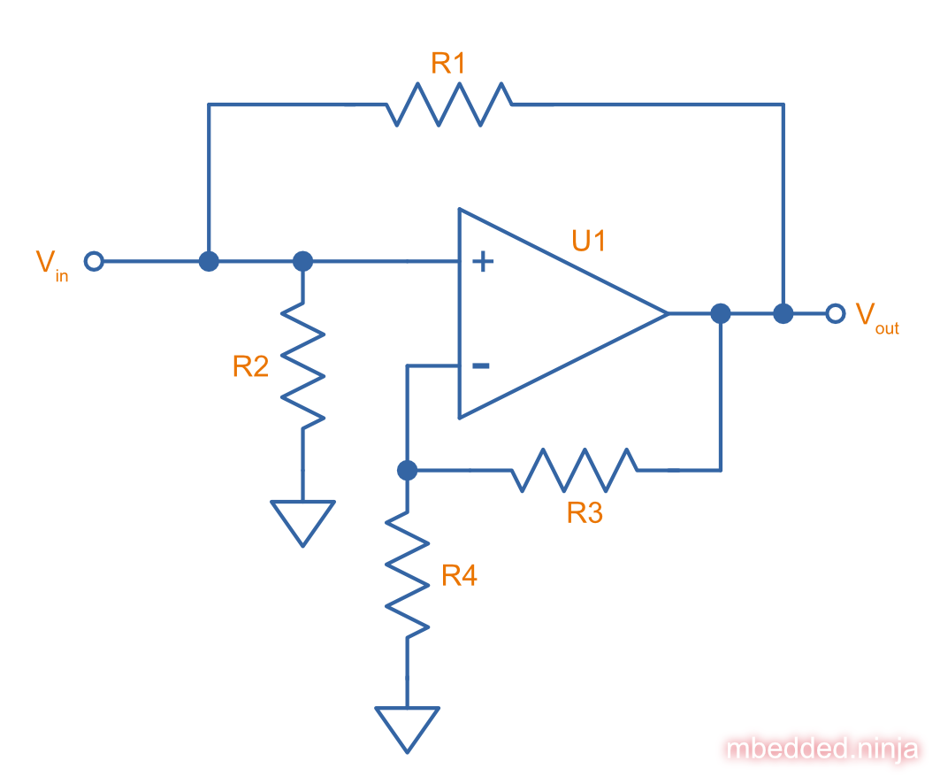
At frequencies much higher than the cut-off , we can assume the two capacitors are shorts. This gives us the schematic in This is a placeholder for the reference: fig-high-pass-variable-gain-sallen-key-filter-freq-limit.
If we assume a non-infinite open-loop gain of the op-amp, the transfer function of this above circuit is:
where is the feedback factor (how much of the output is fed back to the inverting terminal via the voltage divider made from and ):
If we divide the numerator and denominator of by the behaviour of the transfer function as drops becomes more apparent:
When the open-loop gain is large, this equation just becomes , the standard gain equation for a non-inverting op-amp. However, as decreases we can no longer ignore the term and it starts reducing the overall gain of the circuit.
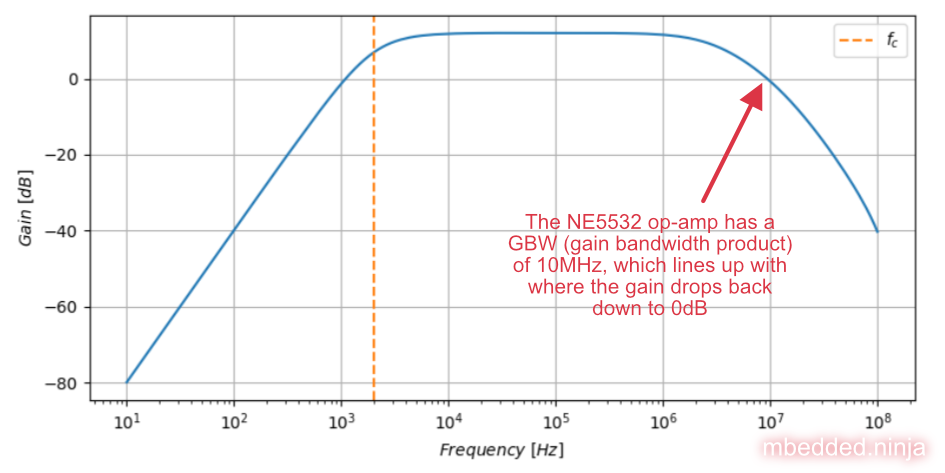
You can see a practical example of this frequency limitation with the high-pass Sallen-Key filter we designed above. As shown in This is a placeholder for the reference: fig-high-pass-sallen-key-fc2khz-q0.8-k4-freq-limitation-plot, the gain of the high-pass filter starts falling and hits at the stated gain bandwidth product at .
Interactive Sallen-Key Designer
The widget below lets you design or analyse a 2nd-order Sallen-Key filter directly in the browser. In Design mode, enter a target cut-off frequency, quality factor and gain, and it solves the equations above for real components (snapping the resistors to the nearest E96 values). In Analyse mode, enter your component values and it reports the resulting , and gain. Either way, the Bode magnitude and phase plots update live, and the peaking discussed above is flagged when it occurs.
Target specification
Components (ideal → nearest E96)
As built (E-series)
Calculators
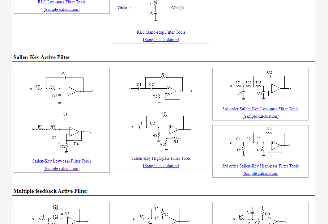
The OKAWA Electric Design website has some good Sallen-Key filter calculators, including 2nd and 3rd-order low-pass and high-pass calculators.
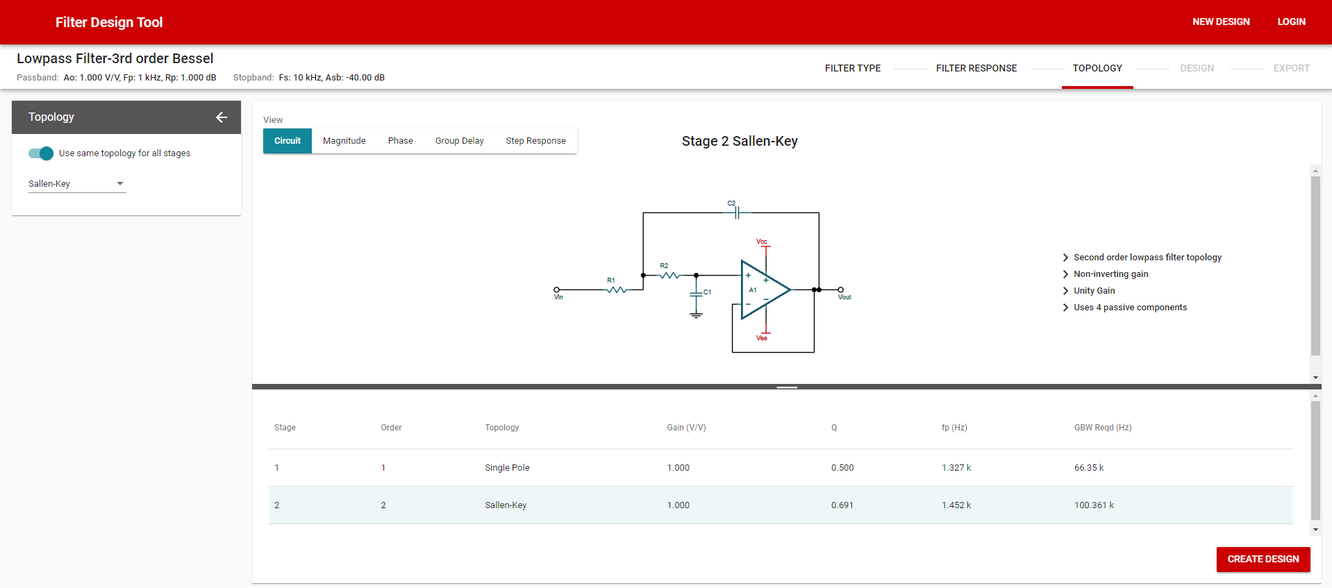
The Texas Instruments Filter Design Tool is a web-based tool that supports the Sallen-Key topology. You firstly enter in the desired characteristics of your filter (e.g. low-pass, cut-off frequency, amount of rejection in stop band, tuning, etc.) and then can select Sallen-Key as a topology to implement the filter with.
Further Reading
For general information on analogue filters, see the Analogue Filters page.
See the Filter Tunings page for information on Butterworth, Bessel, Chebyshev, etc. filter tunings and their polynomial coefficients (these can be applied to a Sallen-Key filter topology).
Footnotes
-
Analog Devices. Chapter 8: Analog Filters. Retrieved 2022-09-20, https://www.analog.com/media/en/training-seminars/design-handbooks/Basic-Linear-Design/Chapter8.pdf. ↩ ↩2 ↩3 ↩4 ↩5 ↩6
-
Jim Karki (2002, Sep). SLOA049B: Active Low-Pass Filter Design. Texas Instruments. Retrieved 2022-09-21, from https://www.ti.com/lit/an/sloa049b/sloa049b.pdf. ↩
-
Ableton. Live Manual - 24. Live Audio Effect Reference. Retrieved 2026-01-24, from https://www.ableton.com/en/live-manual/11/live-audio-effect-reference/. ↩
-
Gary Tuttle. EE 230: Second-order Filters (lecture slides). Retrieved 2022-10-01, from http://tuttle.merc.iastate.edu/ee230/topics/filters/second_order_intro.pdf. ↩
-
Texas Instruments (2021, Jun). SBOA225: Single-supply, 2nd-order, Sallen-Key high-pass filter circuit. Retrieved 2022-09-21, from https://www.ti.com/lit/an/sboa225/sboa225.pdf. ↩
-
OKAWA Electric Design. Filter Design and Analysis (web application). Retrieved 2022-09-29, from http://sim.okawa-denshi.jp/en/Fkeisan.htm. ↩
-
Texas Instruments. Filter Design Tool (web application). Retrieved 2022-09-29, from https://webench.ti.com/filter-design-tool/filter-type. ↩