What Are Transfer Functions, Poles, And Zeroes?

Article by:

Date Published:	September 4, 2021
Last Modified:	October 26, 2022

Overview

Transfer functions are a way of describing the frequency and phase response of a LTI (linear time invariant) system. The system can be anything with a measurable input and output, e.g. mechanical spring/mass/dampers, electronic RLC circuits, e.t.c. This page will put an emphasis on electrical transfer functions in the continuous-time domain.

The Laplace Domain

Transfer functions are usually written in the Laplace domain using the variable $s$, where $s$ is equal to:

$$\begin{align} s = \sigma + j\omega \end{align}$$

where:
$\sigma$ is the real part which determines the exponential increase/decrease
$j$ is the imaginary number ($j = \sqrt{-1}$), also seen as $i$ in maths ($j$ is used in electronics as to not get $i$ confused with current)
$\omega$ is the angular frequency, in units $rads^{-1}$. Remember that $\omega = 2{\pi}f$

NOTE

Angular frequency $\omega$ $[rads^{-1}]$ is used rather than standard frequency $f$ $[Hz]$ just to keep the equations tidier, but it is trivial to convert from one to the other!

Because we normally only care about what happens to steady-state sinusoidal signals (i.e. transients have all died away), we can simplify the equation by setting $\sigma = 0$, as $\sigma$ encodes the exponentially increasing/decaying components. This is essentially simplifying the general Laplace transform to the simpler Fourier transform, and thus $s$ becomes:

$$\begin{align} \label{eq:s-eq-j-w} s = j\omega \end{align}$$

Transfer functions describe the relationship between output and input (typically of voltage, but it doesn’t have to be). $Eq.\ \ref{eq:xfer-fn-vout-vin}$ shows this relationship. We will use the symbol $H(s)$ is represent the transfer function (we are referring to a continuous-time system here, you might see $H(z)$ used for a discrete-time system).

$$\begin{align} \label{eq:xfer-fn-vout-vin} H(s) = \frac{v_{out}(s)}{v_{in}(s)} \end{align}$$

The above equation is great, but is really just one of those “be definition” equations and doesn’t tell you anything about an electrical system (e.g. filter). The real usefulness comes in when you can write $\frac{v_{out}(s)}{v_{in}(s)}$ in terms of the circuit components, typically using KVL/KCL. This lets you write the transfer function with a polynomial on top and bottom:

$$\begin{align} H(s) = \frac{6s}{s^2 + 2s + 9} \end{align}$$

This is much more useful! It tells use everything we need to know about the electrical system (more on this below).

Magnitude and Phase

Note that because we are using the complex variable $s$, the transfer function $H(s)$ encodes both magnitude and phase relationships between the output and input. On it’s own, it’s complex in nature and not really useful for deducing anything “measurable”. But, using two clever tricks, you can separately extract the magnitude and phase response equations from $H(s)$. The below diagram shows the value of $H(s)$ at a single frequency $\omega$, and how the magnitude and phase information is encoded in this (more on this below).

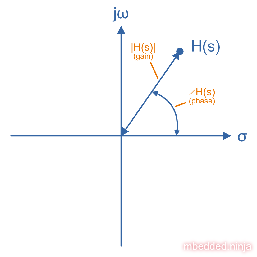
Bear in mind that the above plot shows $H(s)$ at a single frequency. This point will move around as the frequency changes. The magnitude response is found by taking the magnitude of $H(s)$, which is $|H(s)|$ as shown in $Eq.\ \ref{eq:xfer-fn-magnitude}$.

$$\begin{align} \label{eq:xfer-fn-magnitude} | H(s) | = \left| \frac{v_{out}(s)}{v_{in}(s)} \right| \end{align}$$

You might see the magnitude (gain) written as $G(\omega)$. This is equivalent to the magnitude of $H(s)$, i.e.:

$$\begin{align} | H(s) | = G(\omega) \end{align}$$

A $\omega$ is used with $G$ for the gain rather than $s$ because the process of taking the magnitude of $H(s)$ removes all imaginary components, leaving a function which is just dependent on $\omega$ and not $j\omega$.

To calculate the magnitude of the numerator and denominator, you generally:

Substitute in $j\omega$ for $s$ into the polynomials on the top and bottom of the transfer function.
Simplify any $j$’s that are now risen to powers. For example, $j^2 = -1$, $j^3 = -j$, e.t.c.
Group all the real components together, and group all the imaginary components together, so it’s in the form $a + jb$.
Now that we’ve grouped the real and imaginary components, we can use the rule $| a + jb | = \sqrt{a^2 + b^2}$. This removes the imaginary component from the equation.
Simplify as needed.

TIP

Sometimes you’ll see the equation for calculating the magnitude of an complex number as:

$$\begin{align} |a + jb| = \sqrt{(a + jb)(a - jb)} \end{align}$$

This is equivalent to $| a + jb | = \sqrt{a^2 + b^2}$, but in my opinion it takes more simplifying, so I prefer the simple square-root-of-squares approach (which is also intuitive to remember). Remember that the magnitude is the distance of the complex number from the origin when drawn on the complex plane, so you can use Pythagoras’ theorem.

The phase response $\angle H(s)$ is found by finding the angle of the complex number from the positive x-axis, as shown in $Eq.\ \ref{eq:xfer-fn-phase}$.

$$\begin{align} \label{eq:xfer-fn-phase} \angle H(s) &= Arg{\left(\frac{\Im \{H(s)\}}{\Re \{H(s)\}}\right)} \end{align}$$

where:
$Arg$ is the argument (implemented with $atan2(y, x)$ in many software packages)
$\Im\{H(s)\}$ is the imaginary part of $H(s)$
$\Re\{H(s)\}$ is the real part of $H(s)$

WARNING

Using $tan^{-1}$ ($\arctan$) to calculate the angle can sometimes be wrong, as this function throws away information about sign. You have to be aware of what quadrant of the Argand diagram you are in and compensate appropriately. Or stick to using an atan2(y, x) function if your calculator/programming language supports it, as this does all the hard work for you.

Rather than finding the imaginary and real parts of the entire transfer function to calculate the phase, it can be easier to work out the real/imaginary parts for the numerator/denominator separately:

$$\begin{align} \angle H(s) = \angle (numerator) - \angle (denominator) \end{align}$$

$\angle H(s)$ is sometimes written as $\theta(\omega)$. When calculating the phase response it removes the imaginary components of the complex numbers and you’re left with an angle that is a function of just $\omega$.

Poles and Zeroes

A value of $s$ that causes the a transfer function to be 0 is called a zero, and a value of $s$ that causes the transfer function to be infinite is called a pole. Zeroes generally occur when a factor in the numerator is 0 (one notable exception is that a zero can also occur as $s \rightarrow \infty$, if the denominator is of higher order than the numerator), poles generally occur when a factor in the denominator is 0. Poles that have an imaginary component always come in pairs (conjugate pairs).

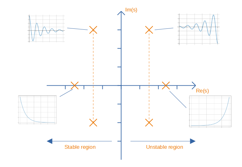
Intuitively, you can think of zeroes as places in where the system completely blocks a certain frequency (as the numerator goes to 0, so does the entire function). A poles is a frequency where the system has infinite response (at least mathematically, as the denominator goes to 0, the function goes to infinity). Poles in the right-half of the Argand diagram (which have a positive real component) cause the system to diverge towards infinity, and your system will be unstable.

TIP

A notable exception to the rule off “all poles must have a negative real component” is for oscillators. You want them to have some positive feedback, that’s what makes them oscillate by themselves!

The zeroes are the roots of the numerator polynomial, and the poles are the roots of the denominator polynomial. For this reason they are also referred to generally as roots.

The poles and zeros of a system can tell you much about how the system performs – it can tell you if the system is stable, and how fast it responds. In fact, the poles and zeroes completely characterize the filter, except for the overall gain constant $K$¹.

For example, the transfer function in $Eq. \ref{eq:xfer-fn-1-over-s}$ has a pole at the origin and a zero at infinity. This simple transfer function represents an integrator. A constant voltage applied to it will result in an output climbs without any limit. However, at high frequencies, the output is essentially zero as the positive and negative parts of the waveform are averaged out over time.

$$\begin{align} \label{eq:xfer-fn-1-over-s} H(s) = \frac{1}{s} \end{align}$$

Pole Zero Plots (Argand Diagrams)

Poles and zeroes are plotted in a Argand diagram in what is called a pole-zero plot to give the reader an understanding on how the circuit responds.

Zeroes contribute +90 of phase and increase the magnitude, above the zero frequency.
Poles contribute -90 of phase and decrease the magnitude, above the pole frequency.

Poles are normally drawn as X’s on the graph, and zeroes as O’s. Unless you are building an oscillator, poles in the right-hand half of the plane (having a positive real component) are a bad thing, as they represent an instability.

Argand diagram showing how the location of poles (no zeroes shown) on a pole zero plots shows how components of the system respond to transients (i.e. impulses).

Group Delay

The group delay $D(\omega)$ is defined as the negative of the slope of the phase vs. frequency plot. This can be written mathematically as:

$$\begin{align} D(\omega) \triangleq -\frac{d}{d\omega} \theta(\omega) \end{align}$$

where:
$\theta(\omega)$ is the phase response of the filter, also written as $\angle H(s)$

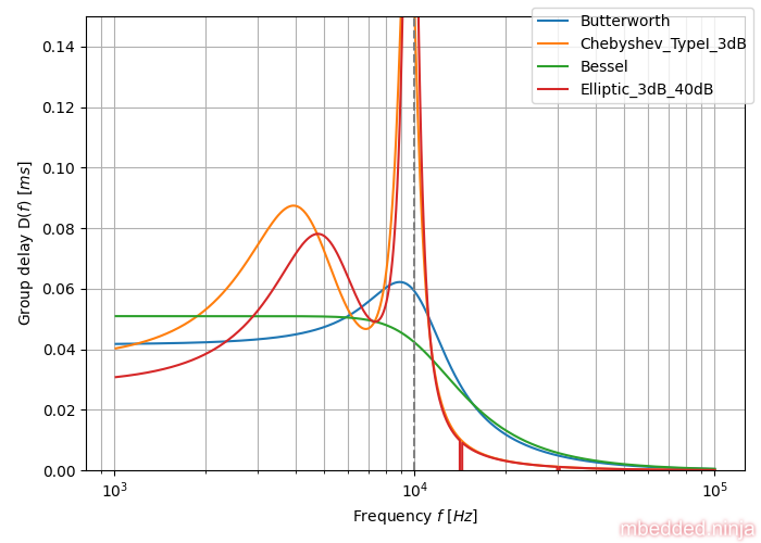
Intuitively, you can think of group delay as the time delay in seconds that a signal takes to pass through a filter as a function of frequency. Group delay has units of seconds. All casual filters (e.g. analogue filters) will have a non-zero, positive group delay. “Flatish” group delay plots in the passband are generally desirable as this means all frequencies will take the same time to pass through the filter, and thus the signal at the output will have minimal distortion (distortion is a result of different frequencies being delayed for different amounts of time).

Group delay for a number of 4-order filter tunings is shown below. The Bessel filter tuning aims to have maximally flat group delay across the pass-band of the signal (at the expense of other metrics we don’t talk about here). You can see this in the plot with the straight green line.

Group delay plotted for a number of different 4-order filter tunings.

Group delay can be calculated in Python with scipy. scipy provides the scipy.signal.group_delay() function which takes as input the numerator and denominator coefficients of the transfer function and returns the calculated group delay.

The Transfer Function Of A Low-Pass RC Filter

A first-order low-pass RC filter has the transfer function shown in $Eq.\ \ref{eq:rc-xfer-fn}$.

$$\begin{align} \label{eq:rc-xfer-fn} H(s) &= \frac{1}{1 + \b{s}RC} \end{align}$$

Using $Eq.\ \ref{eq:s-eq-j-w}$, we can replace $s$ with $j\omega$ to get $Eq.\ \ref{eq:rc-xfer-fn-jw}$.

$$\begin{align} \label{eq:rc-xfer-fn-jw} H(\omega) &= \frac{1}{1 + j\omega RC} \end{align}$$

This system has a pole at $\omega = -\frac{1}{jRC} = \frac{j}{RC}$ and a zero at $\omega = \infty$.

We can find the magnitude response of this low-pass RC filter by taking the magnitude of $H(f)$, remembering that the magnitude of a complex number is defined as:

$$\begin{align} \label{eq:magnitude-of-complex-num} |a + jb | = \sqrt{a^2 + b^2} \end{align}$$ $$\begin{align} \label{eq:abc} | H(\omega) | &= \left| \frac{1}{1 + j\omega RC} \right| \nonumber \\ &= \frac{1}{\sqrt{(1 + j\omega RC)(1 - j\omega RC)}} \nonumber \\ &= \frac{1}{\sqrt{1 - (j\omega RC)^2}} \nonumber \\ &= \frac{1}{\sqrt{1 - (-1)(\omega RC)^2}} \nonumber \\ \label{eq:mag-response-lp-rc-filter} &= \frac{1}{\sqrt{1 + (\omega RC)^2}} \\ \end{align}$$

$Eq. \ref{eq:mag-response-lp-rc-filter}$ shows the final result. Notice that by finding the magnitude, the imaginary components are gone! We can plot this on a graph.

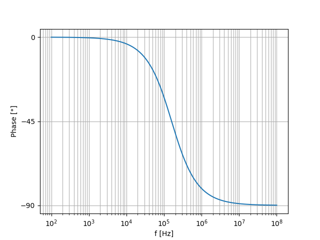
The magnitude response of the the low-pass RC filter, found by plotting $Eq.\ \ref{eq:mag-response-lp-rc-filter}$. Note that the magnitude has been converted into decibels with $dB = 20log10(mag)$.

We can find the phase response of the low-pass RC filter by using rule in $Eq.\ \ref{eq:xfer-fn-phase}$.

$$\begin{align} \angle H(j\omega) &= Arg\left(H(j\omega)\right) \nonumber \\ &= Arg\left(\frac{1}{1 + j\omega RC}\right) \nonumber \\ &= Arg(1) - Arg(1 + j\omega RC) \nonumber \\ &= 0 - arctan\left(\frac{j\omega RC}{1}\right) \nonumber \\ \label{eq:phase-response-lp-rc-filter} &= -arctan\left(j\omega RC\right) \\ \end{align}$$

TIP

We can safely reduce $Arg$ to $arctan$ because we know that $1 + j\omega RC$ will be in the 1st quadrant of the Argand diagram for all positive real values of $\omega$.

The phase response of the the low-pass RC filter, found by plotting $Eq.\ \ref{eq:phase-response-lp-rc-filter}$

Transfer Function Design Tools

Wolfram Alpha

Wolfram Alpha can take a transfer function and calculate many of it’s properties. It recognises the keywords transfer function in front of the numerator/denominator. For example, if you input in it’s search bar (which is a 2nd-order Bessel-tuned filter):

1
transfer function (3)/(s^2+3s+3)

It will spit back at you things like the unit step response, state space representation, zeroes and poles, bode plot, Nyquist plot, Nichols plot, Root locus plot, gain margin and phase margin². Click here to jump to these results in Wolfram Alpha.

Screenshot of Wolfram Alpha's results when you provide it a transfer function[^bib-wolfram-alpha-transfer-function-2nd-order-bessel]. — Screenshot of Wolfram Alpha’s results when you provide it a transfer function².

OKAWA Transfer Function Analysis and Design Tool

The OKAWA Electric Design website has a Transfer Function Analysis and Design tool which can calculate many of the same things the Wolfram Alpha tool can³.

References

MIT: Department of Mechanical Engineering. 2.14 Analysis and Design of Feedback Control Systems: Understanding Poles and Zeros. Retrieved 2022-10-24, from https://web.mit.edu/2.14/www/Handouts/PoleZero.pdf. ↩︎
Wolfram Alpha. Results from providing the input text “transfer function (3)/(s^2+3s+3)”. Retrieved 2022-10-22, from https://www.wolframalpha.com/input?i=transfer+function+%283%29%2F%28s%5E2%2B3s%2B3%29. ↩︎ ↩︎
OKAWA Electric Design. Transfer Function Analysis and Design Tool. Retrieved 2022-10-23, from http://sim.okawa-denshi.jp/en/dtool.php. ↩︎

Authors

Geoffrey Hunter

Dude making stuff.

Twitter

GitHub

This work is licensed under a Creative Commons Attribution 4.0 International License .