Probabilities

Probability Density Functions (PDFs)

This is the graph you’ll typically see when talking about distributions, for example the classic Normal (Gaussian) distribution:

The PDF of the normal distribution, with $\mu=0$ and $\sigma=1$. The x-axis has been cut-off at the 1% and 99% percentiles, in reality the function continues from negative infinity to positive infinity.

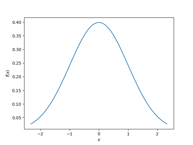
This site uses the notation $f(x)$ to represent the probability density function of $x$.

$$\begin{align} P(a \le x \le b) = \int_a^b f(x) dx \end{align}$$

Cumulative Density Function (CDFs)

The cumulative density function (CDF) is a function which gets a PDF and for any x, cumulatively sums up the probability up to that point. The y-axis always starts a $0$ and ends at $1$.

The CDF of the normal distribution, with $\mu=0$ and $\sigma=1$. The x-axis has been cut-off at the 1% and 99% percentiles, in reality the function continues from negative infinity to positive infinity. The PDF of this distribution is shown in [^pdf-normal].

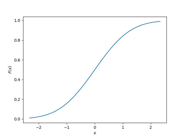
This site uses the notation $F(x)$ to represent the cumulative density function of $x$.

$$\begin{align} F(x) = P(X \le x) \end{align}$$

Quantile Function

The quantile function is the inverse of the cumulative density function (CDF). Also called the percentage point function (PPF) or ICDF (inverse cumulative density function).

The quantile function of the normal distribution, with $\mu=0$ and $\sigma=1$. The x-axis has been cut-off at the 1% and 99% percentiles, in reality the function continues from negative infinity to positive infinity. The PDF of this distribution is shown in [^pdf-normal].

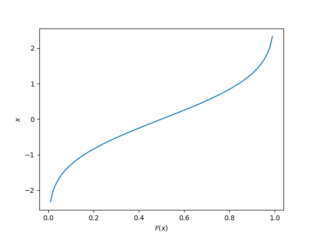
The quantile function is a great way of generating random numbers that follow a specific distribution. Starting with uniformly distributed random numbers in the range from $0$ to $1$ (which is trivially easy to do in most programming languages), you can transform these numbers with the quantile function into random numbers which follow your specific probability distribution.

Generating Random Numbers That Follow A Custom PDF

This section shows you how you can generate an arbitrary number of random numbers that follow a specific distribution. The distribution is defined by a probability density function (all though you could quite as easily define it by the CDF or quantile function). The code example is done in Python.

Let’s define a custom PDF. For this example I just used sin(x) in the range from 0 to pi, but it could be anything you want. Make sure that you scale the PDF so that the total area under the curve is 1 (i.e. divide the function by it’s integral, see the code below for how this is done):

from scipy import integrate
from scipy.interpolate import interp1d
from scipy import stats

# Make up a example PDF
pdf_x = np.linspace(0, np.pi)
pdf_y = np.sin(pdf_x)

Now let’s normalize the PDF so the total area under the curve is 1:

# Normalize pdf_y (make area = 1)
pdf_y_interp = interp1d(pdf_x, pdf_y, kind='cubic')
integral, _ = integrate.quad(pdf_y_interp, 0, np.pi)
pdf_y = pdf_y / integral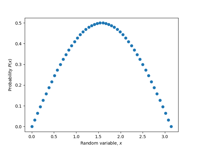

A plot of the “custom” PDF we are going to use to define the distribution to generate random numbers from. In this example I just used sin(x) in the range of 0 to pi.

Now find the quantile function (PPF):

discrete_cdf1 = integrate.cumtrapz(y=pdf_y, x=pdf_x, initial=0)
cdf1 = interp1d(pdf_x, discrete_cdf1)
ppf1 = interp1d(discrete_cdf1, pdf_x, bounds_error=False, fill_value=np.NaN, kind='cubic')

class Dist(stats.rv_continuous):
    def _cdf(self, x):
        return cdf1(x)

    def _ppf(self, x):
        return ppf1(x)

Now lets generate some random numbers!

dist = Dist(a=pdf_x[0], b=pdf_x[-1], xtol=1e-6)

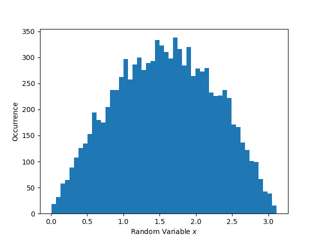
# Now generate 10,000 random values that follow the distribution as specified by your PDF
random_values = dist.rvs(size=10000)

Histogram showing the distribution of the 10,000 generated random numbers:

A histogram of 10,000 generated random numbers that follow the distribution defined by our PDF. Notice how it closely follows the PDF defined in [^generating-rvs-starting-pdf], but with random “jitter” as you would expect if generating numbers randomly.

from scipy import integrate
from scipy.interpolate import interp1d
from scipy import stats

# Make up a example PDF
pdf_x = np.linspace(0, np.pi)
pdf_y = np.sin(pdf_x)
# Normalize pdf_y (make area = 1)
pdf_y_interp = interp1d(pdf_x, pdf_y, kind='cubic')
integral, _ = integrate.quad(pdf_y_interp, 0, np.pi)
pdf_y = pdf_y / integral

discrete_cdf1 = integrate.cumtrapz(y=pdf_y, x=pdf_x, initial=0)
cdf1 = interp1d(pdf_x, discrete_cdf1)
ppf1 = interp1d(discrete_cdf1, pdf_x, bounds_error=False, fill_value=np.NaN, kind='cubic')

class Dist(stats.rv_continuous):
    def _cdf(self, x):
        return cdf1(x)

    def _ppf(self, x):
        return ppf1(x)

dist = Dist(a=pdf_x[0], b=pdf_x[-1], xtol=1e-6)

# Now generate 100,000 random values that follow the distribution as specified by your PDF
random_values = dist.rvs(size=10000)

Generating Random Points On A Sphere

For many different applications, you might find yourself needing to generate random points on a sphere, with the condition that they must be uniformly distributed. You then might think you could do this by using spherical coordinates and:

. Randomly picking a value for $\theta$ (polar angle, measured from the positive Z-axis) between $0$ and $\pi$. . Randomly picking a value for $\phi$ (azimuthal angle)

However, this does not give points that are uniformly distributed! You will find that points will be clustered closer together at the poles of the sphere.

Instead of being uniform, the PDF for $\theta$ (which we will label $f(\theta)$) needs to be proportional to a sine curve, where¹:

$$\begin{align} f(\theta) = \frac{\sin(\theta)}{2} \end{align}$$

References

Footnotes

1. Simon, C. (2015, Feb 27). Generating uniformly distributed numbers on a sphere. Mathemathinking. Retrieved 2021-08-08, from http://corysimon.github.io/articles/uniformdistn-on-sphere/ ↩