Windowed Moving Average Filters

Article by:

Date Published:	February 26, 2014
Last Modified:	May 25, 2022

Overview

Windowed moving average filters are a family of filters which have a finite impulse response (FIR). They all use a finite-length window of data points to calculate the averaged output. The easiest moving average filter to understand is the Simple Moving Average (SMA) filter (also called a box-car filter), which uses a window in where all the inputs values are weighted equally (coefficients are equal). Other moving average filters include the Windowed Exponential Moving Average (EMA) filter, with exponentially-weighted coefficients.

NOTE

“Exponential Moving Average” can also refer to a non-windowed IIR filter, so we are explicit can call this the “Windowed Exponential Moving Average” filter.

Terminology

First off, some terminology.

Window Size (N)

Symbol: $N$

The window size is number of data points used in a moving average filter. $M$ is another letter commonly used to represent the same thing.

Normalized Frequency (F)

Symbol: $F$

The normalised frequency, with units $Hz/sample$. This describes an frequency component in a filter relative to the sampling frequency (e.g. a normalized frequency $F$ of 0.1 means there are 10 samples per cycle. The signal is at Nyquist when $F=0.5$. This is a frequency in the discrete time-domain. Do not confuse with $f$ which is a frequency in the continuous time-domain.

To convert from a standard frequency $f$ to a normalized frequency $F$, use the equation:

$$\begin{align} F = \frac{f}{f_s} \end{align}$$

where:
$ F $ is the normalized frequency, in $Hz/sample$
$ f $ is the standard frequency, in $ Hz $
$ f_s $ is the sample rate, in $ Hz $

The normalized frequency can also be expressed in radians, and if so uses the symbol $\omega$. This has the units $radians/sample$.

Frequency (f)

Symbol: $f$

A frequency of a waveform in the continuous time-domain. Do not confuse with $ F $, which is a frequency in the discrete time-domain.

Sampling Frequency ($f_s$)

The sample frequency of a waveform, measured in the continuous time-domain. This parameter is used when you want to convert a input waveform frequency from a continuous time-domain frequency to a normalised discrete time-domain frequency (see more here).

Simple Moving Average Filter

The simple moving average (SMA) filter (a.k.a rolling average filter) is one of the most commonly used digital filters (or averaging device), due to it’s simplicity and ease of use. Although SMA filters are simple, they are first equal (there are other filters that perform as good as, but not better) at reducing random noise whilst retaining a sharp step response. However, they are the worst filter for frequency domain signals, they have a very poor ability to separate one band of frequencies from another¹.

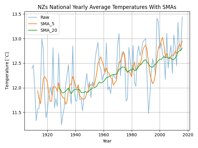
The following plot shows the effect of a SMA filter. The data used is New Zealand’s national average temperature (data from https://data.mfe.govt.nz/table/89453-new-zealands-national-temperature-19092016/):

The effect of SMAs on data. New Zealand's national average yearly temperatures, overlaid with a 5-wide and 20-wide left-handed SMA. — The effect of SMAs on data. New Zealand’s national average yearly temperatures, overlaid with a 5-wide and 20-wide left-handed SMA.

NOTE

Sometimes SMAs don’t start at the same point as the data due to them not being considered “valid” until the window is full of data (like above). Other times you may want to reduce the effective window size as you approach the ends to get an output at every input.

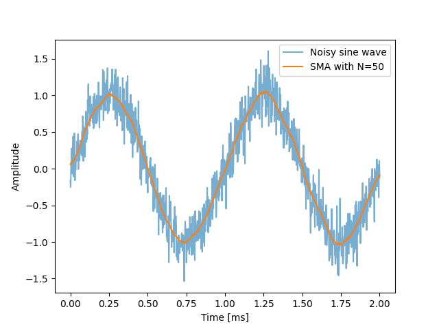
The below plot shows a noisy 1kHz sine wave (with random, normally distributed noise) and then the application of a SMA filter (symmetric, window size = 50) which does a commendable job at recovering the original signal:

Plot showing a noisy sine wave (random, normally distributed noise) and then the application of a SMA filter (symmetric, window size = 50) which recovers the original signal really well!

There are two common types of simple moving average filters:

Left-handed SMA
Symmetric SMA

A left-handed simple moving average filter can be represented by:

$$\begin{align} y[i] = \frac{1}{N} \sum\limits_{j=0}^{N-1} x[i-j] \end{align}$$

where:
$ x $ = the input signal
$ y $ = the output signal
$ N $ = the number of points in the average (the width of the window)

For example, with a windows size of $N = 5$, the moving average at point 9 would be sum of the last 5 inputs $x[9]$ thru to $x[5]$ divided by 5:

$$\begin{align} y[9] = \frac{x[9] + x[8] + x[7] + x[6] + x[5]}{5} \end{align}$$

Left-handed filters of this type can be calculated in real-time ($y[i]$ can be found as soon as $x[i]$ is known).

The window can also be centered around the output signal (a symmetric moving average filter), with the following adjustment of the limits:

$$\begin{align} y[i] = \frac{1}{N} \sum\limits_{j=-(N-1)/2}^{+(N-1)/2} x[i-j] \end{align}$$

For example, using our $y[9]$ again:

$$\begin{align} y[9] = \frac{x[11] + x[10] + x[9] + x[8] + x[7]}{5} \end{align}$$

Symmetric simple moving averages require $N$ to be odd, so that there is an equal number of points either side. The advantage of a symmetric filter is that the output is not delayed (phase shifted) relative to the input signal, as it is with the left-handed filter. One disadvantage of a symmetric filter is that you have to know data points that occur after the point in interest, and therefore it is not real time (i.e. non-casual). Most SMA filters used on stock market data use a left-handed filter so that it is real-time.

When treating a simple moving average filter as a FIR, the coefficients are all equal. The order of the filter is 1 less than the value you divide each value by. The coefficients are given by the following equation:

$$\begin{align} b_i = \frac{1}{N + 1} \end{align}$$

A simple moving average filter can also be seen as a convolution between the input signal and a rectangular pulse whose area is 1.

Frequency Response

The frequency response for a simple moving average filter is given by:

$$\begin{align} H(F) = \frac{1}{N}\frac{sin(\pi F N)}{sin(\pi F)} \end{align}$$

where:
$ H(F) $ is the frequency response
$ F $ the normalised frequency, in $ cycles/sample $
$ N $ = the number of points in the average (the width of the window)

Note that the sine function uses radians, not degrees. You may also see this shown in angular frequency units ($\omega$), in which case $ \omega = 2\pi F $. To convert from a standard frequency $f$ to a normalized frequency $F$, use the equation:

$$\begin{align} F = \frac{f}{f_s} \end{align}$$

where:
$ F $ is the normalized frequency, in $cycles/sample$
$ f $ is the standard frequency, in $ Hz $
$ f_s $ is the sample rate, in $ Hz $

To avoid division by zero, use $ H(0) = 1 $. The magnitude follows the shape of a $ sinc $ function.

The frequency response can also be written as²:

$$\begin{align} H(\omega) = \frac{1}{N}\left(\frac{1 - e^{-j\omega N}}{1 - e^{-j\omega}}\right) \end{align}$$

Lets design a SMA filter with a sampling rate of $1kHz$ and a window size of $10$. This gives the following magnitude response:

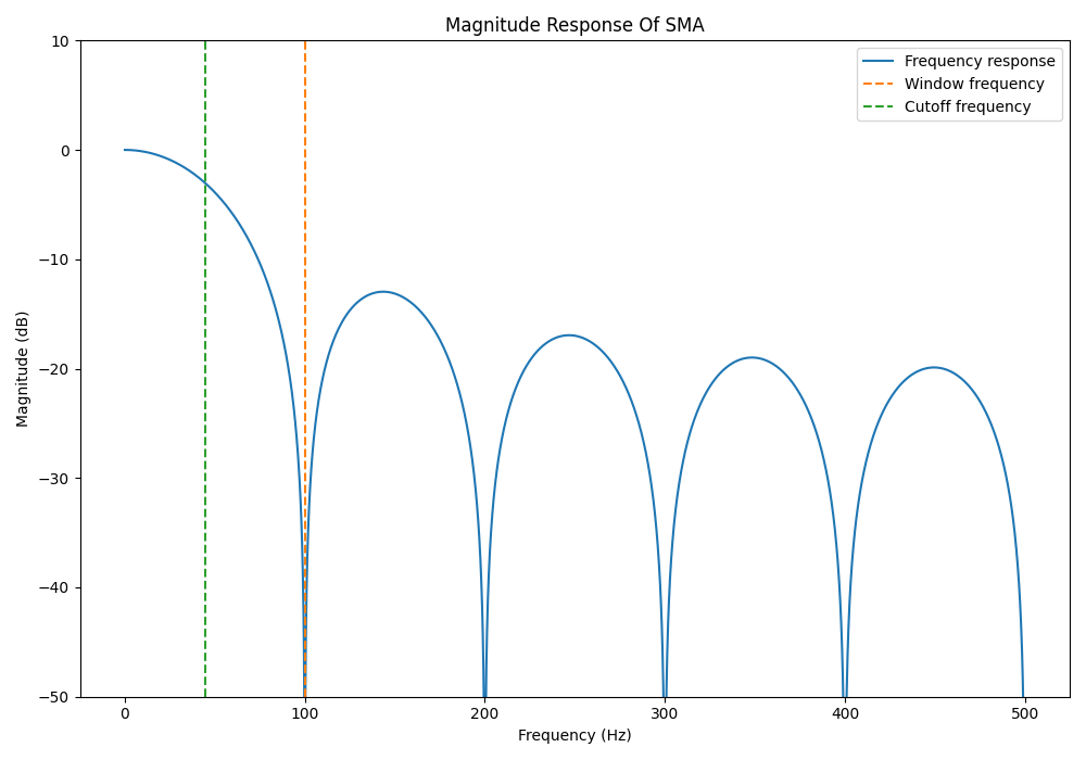
The magnitude response of a SMA filter with fs=1kHz and a window size of 10. Frequency range is from 0Hz up to Nyquist (fs/2).

As expected, this shows us that at DC, the signal is not attenuated at all. As the frequency increases, the filter then begins to block more and more, until it lets through absolutely no signal at $100Hz$. This can be intuitively understood, because with a $1kHz$ sampling frequency and a window size of $10$, a single cycle of a $100Hz$ signal would fit perfectly into the window. Since you take the average of all the values in the window, this top half of the $100Hz$ signal would cancel out perfectly with the bottom half, giving no output. But then, as the frequency further increases, the filter begins to let through some of the signal, as shown by the side lobes. The next point of infinite attenuation is at $200Hz$, which is when 2 cycles of the signal would fit perfectly into the window. This cycle occurs all the way up to Nyquist at $500Hz$.

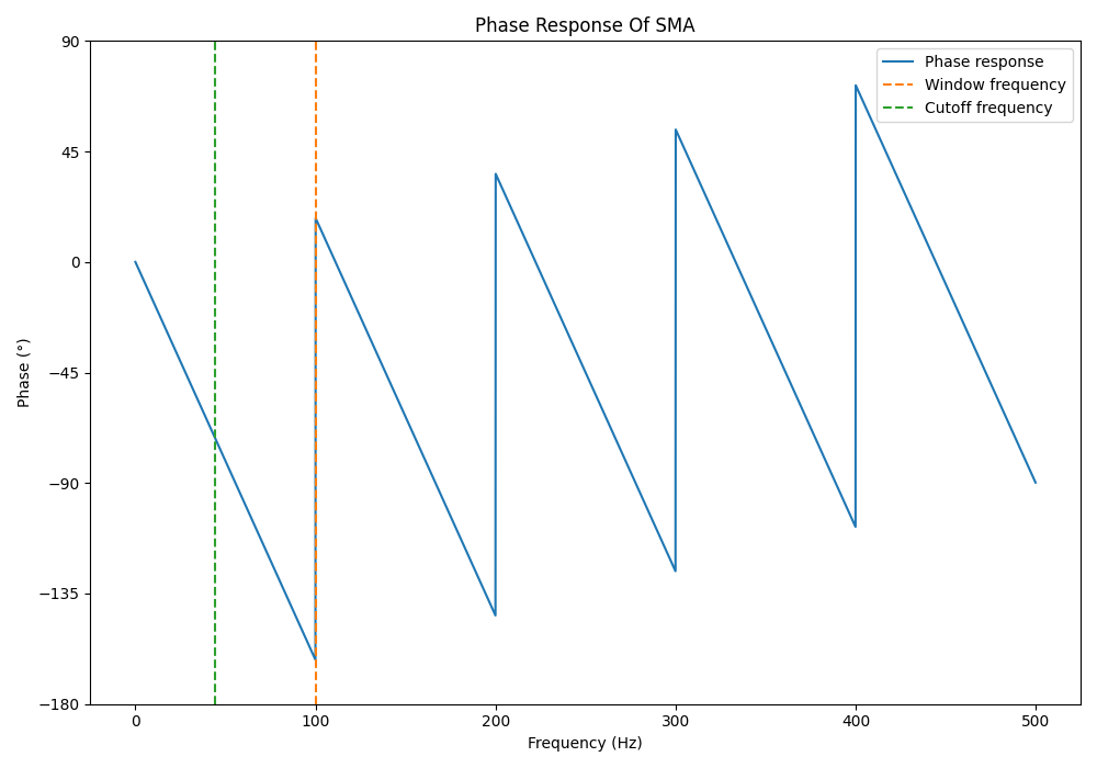
The phase response of the same filter is shown below:

The phase response of a SMA filter with fs=1kHz and a window size of 10. Frequency range is from 0Hz up to Nyquist (fs/2).

For interest, let’s have a look at how increasing the window size effects the frequency response:

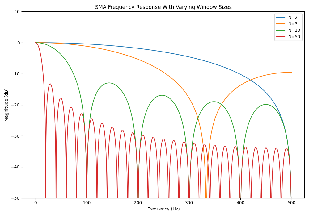
Plot showing what effect an increasing window size has on the frequency response (magnitude) of a SMA filter.

As expected, increasing the window size decreases the cut-off frequency and also improves the roll-off. However, for a left-handed (casual) SMA filter, it also significantly increases the phase shift (or time delay!), so normally a trade-off has to be made.

Cutoff Frequency

When designing a SMA filter, you typically want to set the window size $N$ based on the frequencies you want to pass through and those you want reject. The easiest figure of merit for this is the cutoff frequency $\omega_c$ (or $f_c$), which we’ll define here as the $\frac{1}{2}$ power point ($-3dB$ point). This is the frequency at which the power of the signal is reduced by half.

We can find the equation for the cutoff frequency from $H(\omega)$ above.

\begin{equation} \sin^2 \left(\frac{\omega_c N}{2}\right) - \frac{N^2}{2} \sin^2 \left( \frac{\omega_c}{2} \right) = 0 \end{equation}

Unfortunately, no general closed form solution for the cutoff frequency exists (i.e. there is no way to re-arrange this equation to solve for $\omega_c$). However, these are two ways to get around this problem.

Solve the equation numerically, e.g. use the Newton-Raphson method.
Use an equation which approximates the answer (easier method, recommended approach unless you really need the accuracy!)

Numerically

The Newton-Raphson method can be used to solve the above equation. Below is a code example in Python which includes the function get_sma_cutoff() that can calculate the cutoff frequency $\omega_c$ given the window size $N$ to a high degree of accuracy³:

 1
 2
 3
 4
 5
 6
 7
 8
 9
10
11
12
13
14
15
16
17
18
19
20
21
22
23
import numpy as np
import scipy.signal

def get_sma_cutoff(N, **kwargs):
    """
    Function for calculating the cut-off frequency of a 
    simple moving average filter. Uses the Newton-Raphson method to 
    converge to the correct solution.

    This function was initially written by Pieter P.
    (https://tttapa.github.io/Pages/Mathematics/Systems-and-Control-Theory/
    Digital-filters/Simple%20Moving%20Average/Simple-Moving-Average.html).

    Args:
        N: Window size, in number of samples.

    Returns:
        The angular cut-off frequency, in rad/s.  
    """
    func = lambda w: np.sin(N*w/2) - N/np.sqrt(2) * np.sin(w/2)  # |H(e^jω)| = √2/2
    deriv = lambda w: np.cos(N*w/2) * N/2 - N/np.sqrt(2) * np.cos(w/2) / 2  # dfunc/dx
    omega_0 = np.pi/N  # Starting condition: halfway the first period of sin(Nω/2)
    return scipy.optimize.newton(func, omega_0, deriv, **kwargs)

Approximate Equation

An approximate equation can be found relating the window size to the cutoff frequency which is accurate to 0.5% for $N >= 4$⁴:

$$\begin{align} N = \frac{\sqrt{0.196202 + F_c^2}}{F_c} \end{align}$$

where:
$N$ is the window size, expressed as a number of samples
$F_c$ is the normalized cutoff frequency

Remember that $F_c$ can be calculated with:

$$\begin{align} F_c = \frac{f_c}{f_s} \end{align}$$

where:
$f_c$ is the cutoff frequency, in Hertz $Hz$
$f_s$ is the sample frequency, in Hertz $Hz$

Recursive SMA Implementation

The computation power required to calculate the output at each step in a SMA filter can be significantly reduced with a simple trick. For example, consider a basic left-handed SMA with a window size of 5:

$$\begin{align} y[9] = \frac{x[9] + x[8] + x[7] + x[6] + x[5]}{5} \end{align}$$

Instead of calculating each output as above, we can instead save the last output value we calculated, add the new input data point to it, and subtract the oldest data point from the window:

$$\begin{align} y[9] = y[8] + \frac{1}{5}(x[9] - x[4]) \end{align}$$

This is called a recursive algorithm¹, because the output of one step is used in the calculation of future steps. It’s main benefit is the tremendous speed increase in computing each step, especially when the window size is large. Whilst this dependence on previous output ($y[9]$ depends on $y[8]$) makes it look like an IIR filter, this recursion trick does not change the SMAs behaviour, and it still an FIR filter (once the input flies “past” the end of the window, it has no bearing on the output).

NOTE

The simple moving average filter is the only such window-based filter which can be speed up with this recursion trick. Other forms like exponential, Gaussian and Blackman moving averages have to use computationally expensive convolution.

One thing to watch out for is accumulated error if using floating point numbers. Because you are now calculating the next output value from the previous output calculation (rather than fresh input data, as you would for the non-recursive algorithm), floating point precision errors will accumulate slowly in the output.

To show this, the following graph plots the accumulated error when using 32-bit floating point numbers. 10 million random 32-bit floats in the range of $[0, 1000]$ (our input data) was pushed through a left-handed SMA with a window size of 10 (the window size should not really matter). On every 100th input, the output value as computed by the recursive algorithm was compared with the output computed by the non-recursive algorithm. The difference between these two values is the accumulated error.

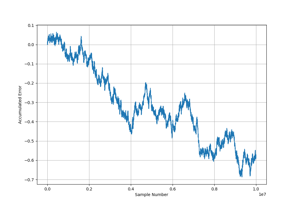
Plot showing the error that slowly accumulates when using the recursive SMA method with floating points.

By the time the 10 million inputs have passed through the filter, the answer is wrong by about 0.6! This may or may not be a bad thing depending on your application. I guess (no proof!) that the average error $e$ will grow proportional to the square root of the number of samples $N$ pushed through the filter, similar to a random walk (drunkards walk).

$$\begin{align} e \propto \sqrt{N} \end{align}$$

WARNING

Watch out when using floating point numbers with the recursive algorithm!

Integer based data does not have this accumulation error problem with the recursive SMA. If you did need to use floats, and you don’t have the CPU brute to use the non-recursive method, one solution may be to periodically clear the previous output value and recompute the output using the non-recursive equation. This will reset your error back to 0, preventing it from growing without bound.

Similarity To Convolution

A SMA filter is identical to the convolution (a mathematical concept) of the input signal with the window waveform (kernel). Typically you would set the height of each point in the window to $\frac{1}{N}$, so that the area under the window curve is 1 (and the SMA has no gain). For example, a 5-point window waveform $g(t)$ would have the values:

$$\begin{align} g(t) = 0, 0, \frac{1}{5}, \frac{1}{5}, \frac{1}{5}, \frac{1}{5}, \frac{1}{5}, 0, 0 \end{align}$$

Multiple Pass Moving Average Filters

A multiple pass simple moving average filter is a SMA filter which has been applied multiple times to the same signal. Two passes through a simple moving average filter produces the same effect as a triangular moving average filter (convolution of a square wave with a square wave is a triangle wave). After four or more passes, it is equivalent to a Gaussian filter¹.

Code Examples

The following code shows how to create a left-handed SMA filter in Python. Note that this example is to show the logic behind the algorithm. For fast and easy SMA use in Python I would recommend using Numpy’s np.convolve() or Panda’s pd.Series.rolling().

 1
 2
 3
 4
 5
 6
 7
 8
 9
10
11
12
13
14
15
16
17
18
19
20
21
22
23
24
25
26
27
28
29
def sma_example_code():
    """
    Example code of recursive left-handed SMA.
    """

    inputs = [1, 6, 3, 4, 2]

    window_length = 3
    moving_average = 0
    window = [0]*window_length
    curr_pos = 0

    for idx, input in enumerate(inputs):
        # Use recursive SMA algorithm
        moving_average = moving_average + 
            (1/window_length)*(input - window[curr_pos])

        # Save new input into window at correct position (overwrite oldest)
        window[curr_pos] = input

        curr_pos += 1
        if curr_pos >= len(window):
            curr_pos = 0
        
        if idx < window_length - 1:
            # SMA not yet valid
            print(f'y[{idx}] = NAN')
        else:
            print(f'y[{idx}] = {moving_average:.2f}')

The output is:

1
2
3
4
5
y[0] = NAN
y[1] = NAN
y[2] = 3.33
y[3] = 4.33
y[4] = 3.00

Fast Start-up

Like all filters, the simple moving average filter introduces lag to the signal. You can use fast start-up logic to reduce the lag on start-up (and reset, if applicable). This is done by keeping track of how many data points have been passed through the filter, and if less have been passed through than the width of the window (i.e. some window elements are still at their initialised value, normally 0), you ignore them when calculating the average.

This is conceptually the same as having a variable-width window which increases from 1 to the maximum value, $x$, as the first $x$ values are passed through the filter. The window width then stays at width $x$ for evermore (or until the filter is reset/program restarts).

If you also know a what times the signal will jump significantly, you can reset the filter at these points to remove the lag from the output. You could even do this automatically by resetting the filter if the value jumps by some minimum threshold.

Exponential Moving Average (EMA) Filters

Unlike a SMA, most EMA filters is not windowed, and the next value depends on all previous inputs. Thus most EMA filters are a form of infinite impulse response (IIR) filter, whilst a SMA is a finite impulse response (FIR) filter. There are exceptions, and you can indeed build a windowed exponential moving average filter in where the coefficients are weighted exponentially.

A exponentially weighted moving average filter places more weight on recent data by discounting old data in an exponential fashion. It is a low-pass, infinite-impulse response (IIR) filter.

It is identical to the discrete first-order low-pass RC filter.

The difference equation for an exponential moving average filter is:

$$\begin{align} y_i = y_{i-1} \cdot (1 - \alpha) + x_i \cdot \alpha \end{align}$$

where:
$ y $ = the output ($i$ denotes the sample number)
$ x $ = the input
$ \alpha $ = is a constant which sets the cutoff frequency (a value between $0$ and $1$)

Notice that the calculation does not require the storage of past values of $x$ and only the previous value of $y$, which makes this filter memory and computation friendly (especially relevant for microcontrollers). Only one addition, one subtraction, and two multiplication operations are needed.

The constant $ \alpha $ determines how aggressive the filter is. It can vary between $0$ and $1$ (inclusive). As $ \alpha \to 0 $, the filter gets more and more aggressive, until at $ \alpha = 0 $, where the input has no effect on the output (if the filter started like this, then the output would stay at $0$). As $ \alpha \to 1 $, the filter lets more of the raw input through at less filtered data, until at $ \alpha = 1 $, where the filter is not “filtering” at all (pass-through from input to output).

The following code implements a IIR EMA filter in C++, suitable for microcontrollers and other embedded devices⁵. Fixed-point numbers are used instead of floats to speed up computation. K is the number of fractional bits used in the fixed-point representation.

 1
 2
 3
 4
 5
 6
 7
 8
 9
10
11
12
13
14
15
16
17
18
19
20
21
22
template <uint8_t K, class uint_t = uint16_t>
class EMA {
  public:
    /// Update the filter with the given input and return the filtered output.
    uint_t operator()(uint_t input) {
        state += input;
        uint_t output = (state + half) >> K;
        state -= output;
        return output;
    }

    static_assert(
        uint_t(0) < uint_t(-1),  // Check that `uint_t` is an unsigned type
        "The `uint_t` type should be an unsigned integer, otherwise, "
        "the division using bit shifts is invalid.");

    /// Fixed point representation of one half, used for rounding.
    constexpr static uint_t half = 1 << (K - 1);

  private:
    uint_t state = 0;
};

Gaussian Window

The 1D Gaussian function $G(x)$ is⁶:

$$\begin{align} \Large G(x) = \frac{1}{\sqrt{2\pi} \sigma} e^{-\frac{x^2}{2\sigma^2}} \end{align}$$

where:
$\sigma$ is the standard deviation

A 5-item symmetric Gaussian window with a standard deviation $\sigma$ of $1$ would give the window coefficients:

1
[ 0.061, 0.245, 0.388, 0.245, 0.061 ]

TODO: Add more info.

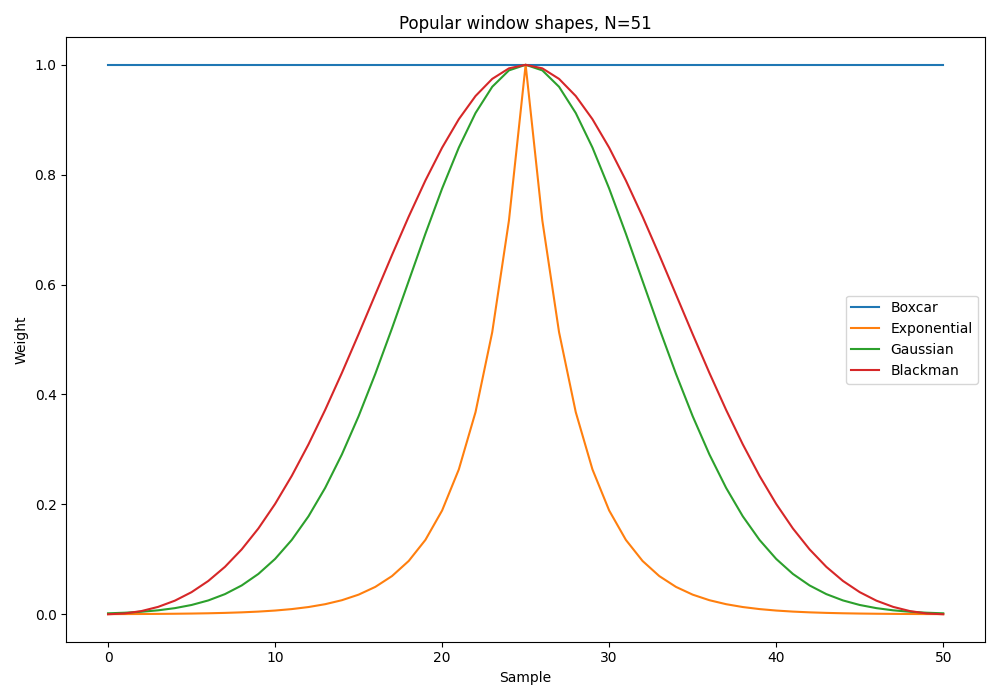
A Comparison Of The Popular Window Shapes

Stuck on what window shape to use? If a simple moving average won’t suffice in it’s simplicity, it might then depend on the frequency response you are after. Popular window shapes and their frequency responses are shown below. All the windows shown below are centered windows (and not left-aligned). The window sample weights are normalized to 1.

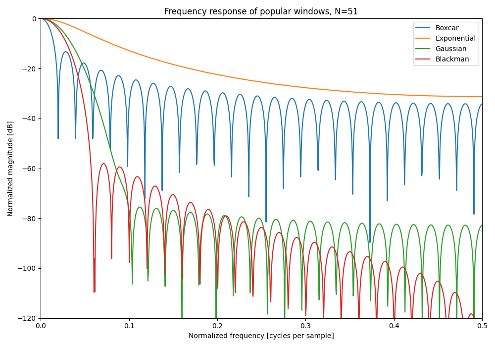
The frequency responses can be found by extending the window waveform with 0’s, and then performing an FFT on the waveform. The resultant frequency domain waveform will be the frequency response of the window. This works because a moving window is mathematically equivalent to a convolution, and convolution in the time domain is multiplication in the frequency domain. Hence your input signal in the frequency domain will be multiplied by FFT of the window.