Filter Tunings

Filter tunings are specific tunings of filters to optimize a particular characteristic of it’s response. Filter tuning directly specifies what the filters polynomials must be in it’s transfer function (see What Are Transfer Functions, Poles and Zeroes for more info).

• Butterworth Optimized for the flattest response through the pass-band, at the expense of having a low transition between the pass and stop-band.
• Chebyshev: Designed to have a steep transition between the pass and stop-band (but not the steepest, Elliptic tuning claims that award), at the expense of gain ripple in either the pass or stopband (type 1 or type 2). Also called Chevyshev, Tschebychev, Tschebyscheff or Tchevysheff, depending on exactly how you translate the original Russian name. There are two types of Chebyshev filters:
  • Type 1: Type 1 Chebyshev filters (a.k.a. just a Chebyshev filter) have ripple in the passband, but no ripple in the stopband.
  • Type 2: Type 2 Chebyshev filters (a.k.a. an inverse Chebyshev filter) have ripple in the stopband, but no ripple in the passband.
• Bessel: Optimized for linear phase response up to (or down to for high-pass filters) the cutoff frequency $f_c$, at the expense of a slower transition to the stop-band. This is useful to minimizing the signal distortion (a linear phase response in the frequency domain is a constant time delay in the time domain).
• Elliptic: Designed to have the fastest transition from the passband to the stopband, at the expense of ripple in both of these bands (Chebyshev optimization only produces ripple in one of the bands but is not as fast in the transition). Also called Cauer filters or Rational Chebyshev filters.

These filters are explained in more detail below. If you are interested in visual comparisons, you can skip straight to the Comparisons Between Filter Tunings section.

Butterworth Tunings

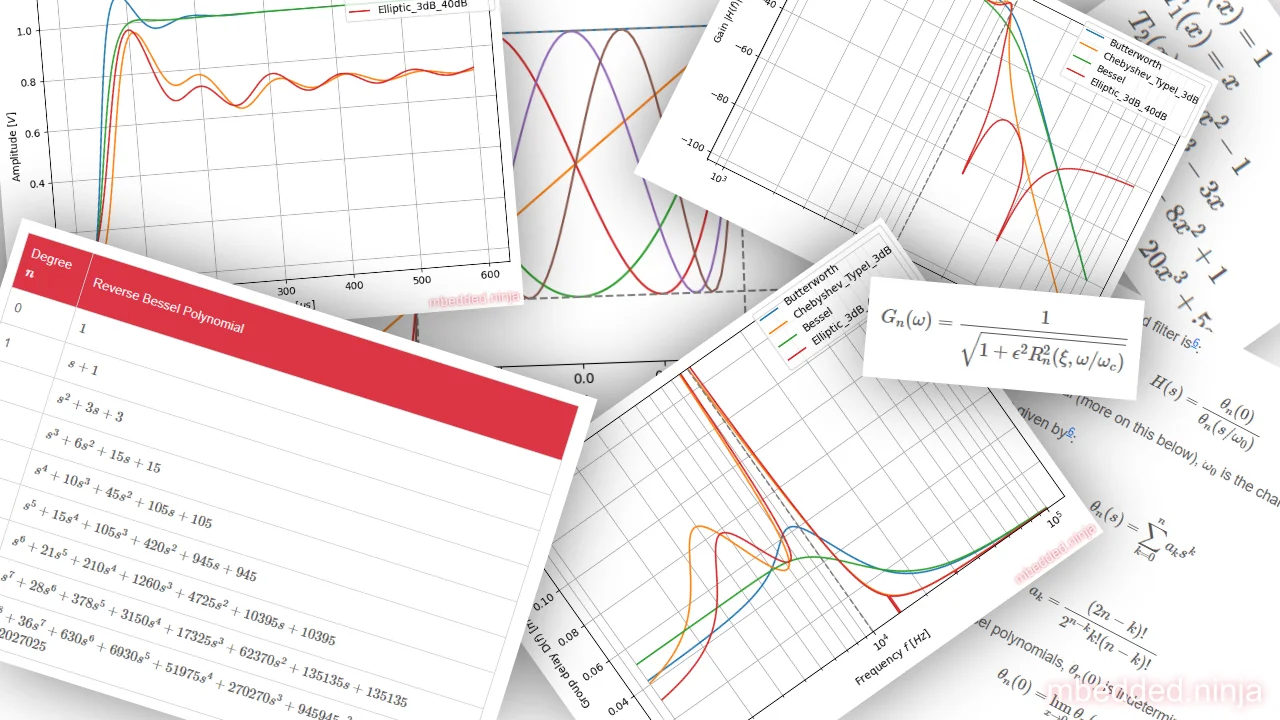
Tuning a filter for a Butterworth response gives a filter which is maximally flat in the passband, and rolls off towards zero in the stopband. The price you pay for this is slower roll-off into the stop-band, compared with Chebyshev or Elliptic tunings.

Tip

It may sound dumb, but I’ve always remembered Butterworth as a flat passband which “slides like butter”.

Butterworth tunings are defined as a filter whose magnitude is¹:

$$\begin{align} | H_n(s) | \triangleq \frac{1}{\sqrt{1 + \omega^\{2n\}}} \end{align}$$

where:
$\omega$ is the angular frequency $[rads^{-1}]$
$n$ is the order of the filter

The normalized Butterworth polynomial of degree $n$ is given by²:

$$\begin{align} B_n(s) = \begin{cases} \prod_{k=0}^{\frac{n}{2} - 1}(s^2 -2\cos{(2\pi\frac{2k + n + 1}{4n})s + 1}) & \text{even }n \\ (s + 1)\prod_{k=0}^{\frac{n - 1}{2} - 1}(s^2 -2\cos{(2\pi\frac{2k + n + 1}{4n})s + 1}) & \text{odd }n \\ \end{cases} \end{align}$$

Tip

If you’ve never seen it before, the uppercase Pi symbol $\prod$ in the above equation represents the product of a series of things, such like the uppercase Sigma symbol $\Sigma$ represents the sum of a series of things. For example, $\prod_{k=1}^{3}k = 1\times 2 \times 3$.

Below is a table of the normalized factored Butterworth polynomials for order $n$. The polynomial is useful in this form as each product forms either a first or second-order partial filter which can be directly implemented by a standard filter topology (e.g. RC filter for a first-order section, Sallen-Key for a second-order section). These polynomials were generated with the Butterworth polynomial equation above. The polynomials are normalized by setting $\omega_c = 1$ (the characteristic frequency).

All numbers are rounded to 3 decimal places.

n	polynomial
1	((s + 1))
2	((s^2 + 1.414 s + 1))
3	(\left(s + 1\right) \left(s^2 + 1.0 s + 1\right))
4	(\left(s^2 + 0.765 s + 1\right) \left(s^2 + 1.848 s + 1\right))
5	(\left(s + 1\right) \left(s^2 + 0.618 s + 1\right) \left(s^2 + 1.618 s + 1\right))
6	(\left(s^2 + 0.518 s + 1\right) \left(s^2 + 1.414 s + 1\right) \left(s^2 + 1.932 s + 1\right))
7	(\left(s + 1\right) \left(s^2 + 0.445 s + 1\right) \left(s^2 + 1.247 s + 1\right) \left(s^2 + 1.802 s + 1\right))
8	(\left(s^2 + 0.39 s + 1\right) \left(s^2 + 1.111 s + 1\right) \left(s^2 + 1.663 s + 1\right) \left(s^2 + 1.962 s + 1\right))

Using these polynomials $B_n$, we can write the transfer function of a Butterworth filter as²:

$$\begin{align} H_n(s) = \frac{1}{B_n} \end{align}$$

Note

This equation is different from Butterworth magnitude equation, because this equation lacks the magnitude $|$ symbols around $H_n(s)$. This equation is the full-and-proper transfer function, which contains both the magnitude and phase information.

This transfer function gives the bode plots in This is a placeholder for the reference: fig-butterworth-bode-plot-for-various-n (by taking the magnitude and arg of the transfer function).

Magnitude and phase bode plots for normalized Butterworth filters of orders 1, 2, 4 and 8.

The Butterworth polynomial coefficients $a_0, a_1, ..., a_n$ for an $n$-order filter can be calculated with this product-based equation¹:

$$\begin{align} a_{k}=\prod _{\mu =1}^{k}{\frac {\cos((\mu -1)\gamma )}{\sin(\mu \gamma )}} \end{align}$$

where:
$a_0 = 1$ (ignore the above equation for $a_0$)
$\gamma = \dfrac{\pi}{2n}$

There is also a recursive formula to calculate the coefficients, but we’ll just use the product based one. The below table shows the Butterworth polynomial coefficients calculated with this equation, up to $n=8$ (8th order filter).

n	polynomial
1	((s + 1))
2	((s^2 + 1.414 s + 1))
3	(\left(s + 1\right) \left(s^2 + 1.0 s + 1\right))
4	(\left(s^2 + 0.765 s + 1\right) \left(s^2 + 1.848 s + 1\right))
5	(\left(s + 1\right) \left(s^2 + 0.618 s + 1\right) \left(s^2 + 1.618 s + 1\right))
6	(\left(s^2 + 0.518 s + 1\right) \left(s^2 + 1.414 s + 1\right) \left(s^2 + 1.932 s + 1\right))
7	(\left(s + 1\right) \left(s^2 + 0.445 s + 1\right) \left(s^2 + 1.247 s + 1\right) \left(s^2 + 1.802 s + 1\right))
8	(\left(s^2 + 0.39 s + 1\right) \left(s^2 + 1.111 s + 1\right) \left(s^2 + 1.663 s + 1\right) \left(s^2 + 1.962 s + 1\right))

For example, the above table tells you for order $n=3$ the Butterworth polynomial is $s^3 + 2s^2 + 2s + 1$. If expand the factorized version we should arrive at the same polynomial:

$$\begin{align} B_3 &= (s + 1)(s^2 + s + 1) \nonumber \\ &= s^3 + s^2 + s + s^2 + s + 1 \nonumber \\ &= s^3 + 2s^2 + 2s + 1 \nonumber \\ \end{align}$$

Yay, they are the same! If you are ever wanting to generate the Butterworth polynomial coefficients yourself, here is a Python function that returns you the Butterworth coefficients for any order $n$:

from typings import List
import numpy as np

def calc_butterworth_coeffs_for_order(n: int) -> List[float]:
    """
    Calculates the Butterworth polynomial coefficients for the given degree n.

    Equation from https://en.wikipedia.org/wiki/Butterworth_filter:
        {\displaystyle a_{k}=\prod _{\mu =1}^{k}{\frac {\cos((\mu -1)\gamma )}{\sin(\mu \gamma )}}\,,}

    Args:
        n   Degree of Butterworth polynomial. Must be >= 0.
    Returns:
        Coefficients of Butterworth polynomial of degree n. Coefficients are returned in a list, in this order: [ a0, a1, ..., an ].
    """

    gamma = np.pi / (2*n)
    # Need to calculate n + 1 coefficients
    coeffs = []
    for k in range(n + 1):
        if k == 0:
            # a_0 = 1.0
            coeffs.append(1.0)
        else:
            # Use product formula
            product = 1.0
            for mew in range(1, k + 1):
                product *= np.cos((mew - 1)*gamma) / np.sin(mew * gamma)
            coeffs.append(product)
    return coeffs

Chebyshev Tunings

Chebyshev-tuned filters with even order numbers (e.g. 2nd order, 4th order, …) generate ripples above the 0dB line, filters with odd order numbers (e.g. 3rd order, 5th order, …) generate ripples below the 0dB line.

Chebyshev-tuned filters can be further broken down into two types:

• Type I: Ripple in the pass-band, no ripple in the stop-band. This is the most common type of Chebyshev-tuned filter, as it has faster roll-off. Sometimes referred to just as a Chebyshev filter (with no mention that it’s Type I).
• Type II: No-ripple in the pass-band, ripple in the stop-band. Also known as an inverse Chebyshev-tuned filter. This is not as popular as Type I as it’s roll-off is not as steep.

Because Chebyshev filters have ripple in the pass-band, their cutoff frequency is usually defined in a completely different way to all other filter optimizations. Rather than specifying $f_c$ as the -3dB point, the $f_c$ for Chebyshev filters is defined at the point at which the gain leaves the allowed ripple region (i.e. > 0.5dB for a 0.5dB Chebyshev filter, > 3dB for a 3dB Chebyshev filter).

A Type I Chebyshev tuned filter of order $n$ has a gain response of³:

$$\begin{align} | H_n(s) | = \frac{1}{\sqrt{1 + \varepsilon^2 T_n(\omega / \omega_0)^2}} \end{align}$$

where:
$\varepsilon$ is the damping factor
$\omega_0$ is the characteristic frequency
$T_n(\omega / \omega_0)$ is a Chebyshev polynomial of the first kind with order $n$

Note

The are actually two different kinds of “Chebyshev polynomials”. In analogue filter design, we always use the first kind (for both Type I and Type II Chebyshev filters), commonly denoted $T_n$. Chebyshev polynomials of the second kind are usually denoted $U_n$.

The ripple in the passband may have multiple maxima and minima. However, the peaks of each maxima/minima have the same amplitude (i.e. they are bounded by a fixed value). This is known as equiripple behaviour, and stems from the core definition of a Type I Chebyshev polynomial.

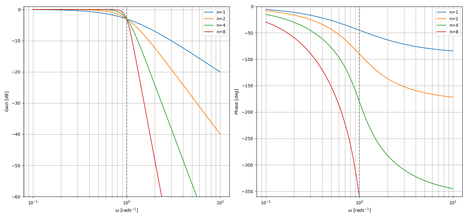
The driving factor behind the Chebyshev tunings is the Chebyshev polynomials of the first kind. They are defined by⁴:

$$\begin{align} T_n(\cos{\theta}) &= \cos(n\theta) \\ \end{align}$$

Tip

It’s a little unusual in the way it’s normally defined with it being a function of $\cos(\theta)$ rather than just $x$. If you let $x = \cos \theta$, then you can substitute $\theta = \arccos x$ are arrive at:

$$\begin{align} T_n(x) &= \cos(n\arccos(x)) \text{ for }|x| \leq 1 \\ \end{align}$$

You can calculate the Chebyshev polynomials of the first kind with the recursive definition⁴:

$$\begin{align} T_0(x) &= 1 \nonumber \\ T_1(x) &= x \nonumber \\ T_{n+1}(x) &= 2xT_n(x) - T_{n-1}(x) \\ \end{align}$$

The first 6 Chebyshev polynomials are shown below:

$$\begin{align} T_0(x) &= 1 \nonumber \\ T_1(x) &= x \nonumber \\ T_2(x) &= 2x^2 - 1 \nonumber \\ T_3(x) &= 4x^3 - 3x \nonumber \\ T_4(x) &= 8x^4 - 8x^2 + 1 \nonumber \\ T_5(x) &= 16x^5 - 20x^3 + 5x \nonumber \\ \end{align}$$

These are special polynomials in which the leading coefficient (coefficient in front of the highest power of $x$) is the largest value it can be whilst the polynomial is bounded between $[-1, 1]$ on the interval $x\ \epsilon\ [-1, 1]$⁴. You can see this interesting behaviour in the graph in This is a placeholder for the reference: fig-chebyshev-poly-graph. It shows the first 6 Chebyshev polynomials $T_0$ through to $T_5$. Note that $T_0 = 1$, and is somewhat hidden by the horizontal bounding line.

The first 6 Chebyshev polynomials (of the first kind) from $T_0$ to $T_5$.

The below Python function can be used to calculate the Chebyshev polynomial coefficients of the first kind, for a given order $n$. Although we could build up a recursive function and use sympy to find them based of the recursive equation above, it’s easier just to use the numpy.polynomial module which provides a function to calculate them.

import numpy.polynomial
def chebyshev_poly_coeffs(n: int) -> List[float]:
    """
    Calculates the Chebyshev polynomial coefficients (of the first kind) for the provided degree n.

    Args:
        n: Degree of polynomial. Must be >= 0.
    Returns:
        List of Chebyshev polynomial coefficients, sorted from lowest degree to highest degree i.e. [ a_0, a_1, ..., a_n ].
    """
    # First build up coefficients for a_0T_0 + a_1T_1 + ... a_nT_n
    input_coeffs = [0] * (n + 1)
    input_coeffs[-1] = 1 # Set the last item to 1, this corresponds to T_n(x)
    # Now convert this to Chebyshev polynomial coefficients
    poly_coeffs = numpy.polynomial.chebyshev.cheb2poly(input_coeffs)
    return poly_coeffs

Bessel Tunings

A Bessel tuned filter is one which has a maximally linear phase response. This corresponds to a maximally flat group/phase delay (the time it takes for a signal to pass through as a function of frequency). This behaviour preserves the shapes of filtered signals in the passband, which is a desirable property for audio signals. It is also sometimes called Bessel-Thomson tuned filters because W. E. Thomson who worked out how to apply Bessel functions to electronic filters in 1949⁵.

The transfer function of a low-pass Bessel tuned filter is⁶:

$$\begin{align} H(s) &= \frac{\theta_n(0)}{\theta_n(s/\omega_0)} \end{align}$$

where $\theta_n(s)$ is a reverse Bessel polynomial (more on this below), $\omega_0$ is the characteristic frequency and $s=k\omega$.

The reverse Bessel polynomials are given by⁶:

$$\begin{align} \theta_n(s) &= \sum_{k=0}^n a_k s^k \end{align}$$

where $a_k$ is a coefficient given by:

$$\begin{align} a_k &= \frac{(2n - k)!}{2^{n-k}k!(n - k)!} \end{align}$$

However, by this definition of the reverse Bessel polynomials, $\theta_n(0)$ is indeterminate. So instead, $\theta_n(0)$ is defined as:

$$\begin{align} \theta_n(0) &= \lim_{x \to 0} \theta_n(x) \end{align}$$

The above equations were used to generate the table below, which lists the reverse Bessel polynomials of degree 0 to 8.

Degree (n)	Reverse Bessel Polynomial
0	(1)
1	(s + 1)
2	(s^2 + 3 s + 3)
3	(s^3 + 6 s^2 + 15 s + 15)
4	(s^4 + 10 s^3 + 45 s^2 + 105 s + 105)
5	(s^5 + 15 s^4 + 105 s^3 + 420 s^2 + 945 s + 945)
6	(s^6 + 21 s^5 + 210 s^4 + 1260 s^3 + 4725 s^2 + 10395 s + 10395)
7	(s^7 + 28 s^6 + 378 s^5 + 3150 s^4 + 17325 s^3 + 62370 s^2 + 135135 s + 135135)
8	(s^8 + 36 s^7 + 630 s^6 + 6930 s^5 + 51975 s^4 + 270270 s^3 + 945945 s^2 + 2027025 s + 2027025)

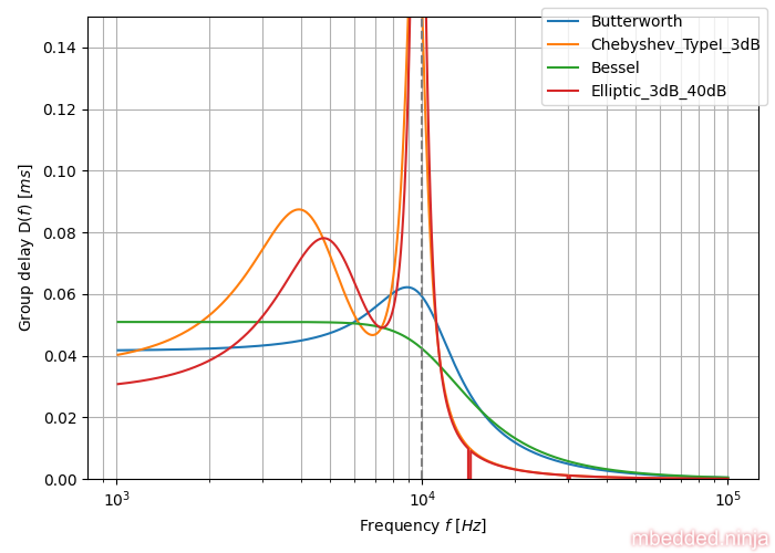
The visually demonstrate the flat group delay of the Bessel tuned filter, we can plot the group delay of the Bessel-tuned 4th-order low-pass filter vs. a number of other popular tunings. The below plot shows the group delay for Bessel, Butterworth, Chebyshev and Elliptic tuned filter. The critical frequency was set to $10kHz$ for all filter tunings. All filters are 4th-order. As you can see in This is a placeholder for the reference: fig-tuning-comparison-group-delay, the Bessel tuned filter has the flattest group delay.

The group delay for various 4th-order filter tunings. The Bessel-tuned filter has the flattest group delay in the passband.

This also means that a Bessel-tuned filter has the least ringing due to a step response, as shown in the plot in This is a placeholder for the reference: fig-tuning-comparison-step-response (more on this in the Comparisons Between Filter Tunings section).

Step response comparison of different filter tunings. The Bessel-tuned filter has the least ringing.

Example

Find the transfer function for a 2nd-order Bessel low-pass filter with $\omega_0 = 1$. Then find the equations for magnitude/phase and create bode plots.

Using the equations or table above, the 2nd-order reverse Bessel polynomial $\theta_2(s/1) = s^2 + 3s + 3$. The limit of this function as $s \to 0$ is $3$. So:

$$\begin{align} H(s) &= \frac{\theta_n(0)}{\theta_n(s/\omega_0)} \nonumber \\ &= \frac{3}{s^2 + 3s + 3} \nonumber \\ \end{align}$$

To find the magnitude response of this we substitute $s = j\omega$.

$$\begin{align} |H(\omega)| &= \left|\frac{3}{(j\omega)^2 + 3(j\omega) + 3}\right| \nonumber \\ &= \frac{3}{|-\omega^2 + 3j\omega + 3|} \nonumber \\ &= \frac{3}{| (3-\omega^2) + j(3\omega) |} \nonumber \\ &= \frac{3}{\sqrt{\omega^4 - 6\omega^2 + 9 + 9\omega^2}} \nonumber \\ &= \frac{3}{\sqrt{\omega^4 + 3\omega^2 + 9}} \nonumber \\ \end{align}$$

And finding the phase response:

$$\begin{align} \angle H(\omega) &= Arg{\left(\frac{\Im \{H(s)\}}{\Re \{H(s)\}}\right)} \nonumber \\ &= Arg{\frac{\Im (num)}{\Re (num)}} - Arg{\frac{\Im (den)}{\Re (den)}} \nonumber \\ &= Arg{\frac{0}{3}} - Arg{\frac{3\omega}{3 - \omega^2}} \nonumber \\ \end{align}$$

$Arg$ can be implemented with atan2() in most programming languages, i.e.:

$$\begin{align} \angle H(\omega) &= Arg{\frac{0}{3}} - Arg{\frac{3\omega}{3 - \omega^2}} \nonumber \\ &= atan2(0,\ 3) - atan2(3\omega,\ 3 - \omega^2) \nonumber \\ \end{align}$$

We now use these equations for magnitude and phase and create bode plots!

Bode plots for the 2nd-order Bessel low-pass filter.

Elliptic Tunings

Elliptic-tuned filters (a.k.a. a Cauer or Zolotarev filter⁷, but not to be confused with the Cauer/ladder filter topology) is a filter that is optimized for the fastest transition in gain from the passband to the stopband. The ripple has constant magnitude in the passband, and the same applies in the stopband (equal ripple)⁸. This does not however mean that the amount of ripple in the passband is the same as what is in the stopband!

Whereas most tunings are defined with a transfer function, the Elliptic filter is a special case where it is defined by it’s gain. The gain for a lowpass Elliptic tuned filter is⁸:

$$\begin{align} G_n(\omega) &= \frac{1}{\sqrt{1 + \epsilon^2 R_n^2 (\xi, \omega/\omega_c)}} \nonumber \\ \end{align}$$

where:
$\epsilon$ is the ripple factor
$R_n(\xi, \omega)$ is the nth-order elliptic rational function
$\xi$ is the selectivity factor ($\xi \geq 1$)
$\omega_c$ is the characteristic frequency, in radians per second $rads^{-1}$

The big problem is that the elliptic ration function $R_n$ cannot be easily expressed algebraically!⁹ It’s general definition involves a Jacobi elliptic cosine function and the elliptic integral⁷. Diving into this would be a headache, so we’re just going to take the easy option and use the Python scipy.signal.ellip() function to provide us with the transfer function coefficients.

You can generate an Elliptical filter in Python using the scipy package:

import scipy.signal

b, a = scipy.signal.ellip(N, rp, rs, Wn, btype='lowpass', analog=True)

where N is the order of the filter, rp is the maximum ripple allowed below unity in the passband, rs is the minimum attenuation required in the stopband, and Wn is the critical (characteristic) frequency. The returned b and a are arrays of the transfer function numerator and denominator coefficients.

Example

Use the Python scipy package and find the transfer function for a 2nd-order lowpass Elliptic-tuned filter with a characteristic frequency of $10kHz$, passband ripple of $3dB$, and a minimum attenuation of $40dB$ in the stopband.

import numpy as np
import scipy.signal
b, a = scipy.signal.ellip(N=2, rp=3, rs=40, Wn=2*np.pi*10e3, btype='lowpass', analog=True)
print(f'b={b}, a={a}')
# b=[1.00098303e-02 0.00000000e+00 1.99828046e+09], a=[1.00000000e+00 4.02295857e+04 2.82264617e+09]

This gives the below transfer function, which considering the coefficients of the other filter tuning types, are pretty strange!

$$\begin{align} H(s) &= \frac{1.00098303\times10^{-2}s^2 + 1.99828046\times10^{9}}{s^2 + 4.02295857\times10^4s + 2.82264617\times10^9} \nonumber \\ \end{align}$$

Caution

You can run into stability issues when representing transfer functions in the b, a form with high-order Elliptic-tuned filters.

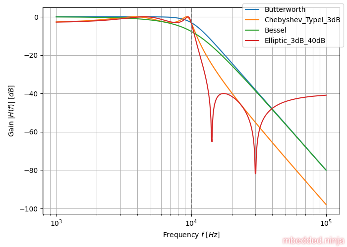
Comparisons Between Filter Tunings

The following parameters were used for the filters:

• All filters are 4th-order filters.
• Characteristic frequency $f_c$ of $10kHz$. For Butterworth and Bessel tunings the characteristic frequency is defined as the $-3dB$ point. For Chebyshev and Elliptic filter tunings the characteristic frequency is defined as the point where the ripple leaves the allowable amount in the passband.
• A rather arbitrary $3dB$ of passband ripple was allowed for both the Chebyshev and Elliptic filters.
• Being even more arbitrary, the Elliptic filter was allowed to rise back up to $-40dB$ in the stopband.

With the above specified, the transfer function of each filter is fully defined.

Now we can finally look at some comparisons. The plot in This is a placeholder for the reference: fig-tuning-comparison-gain-db compares the gain response of each filter tuning. Both axis are logarithmic. You can clearly see the Elliptic-tuned filter winning the race.

Gain comparison of different filter tunings.

I think the difference is gain response can be better viewed with linear x and y axes So we’ll drop the $dB$ in favour of $V/V$ and get rid of the logarithmic x-axis, as shown in This is a placeholder for the reference: fig-tuning-comparison-gain-linear.

Gain comparison of different filter tunings, now with linear x and y axes.

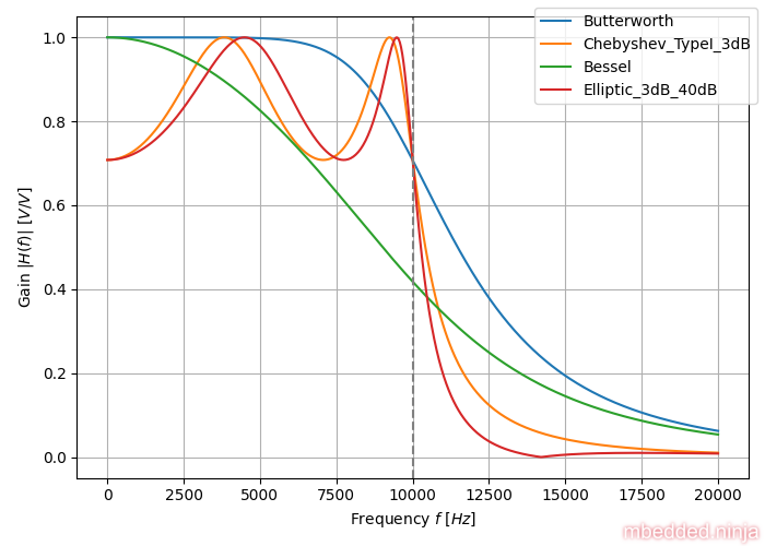
The linear axes helps to highlight the spread in behaviour between the different tunings. Look at that ripple in the passband with the Chebyshev and Elliptic filter tunings!

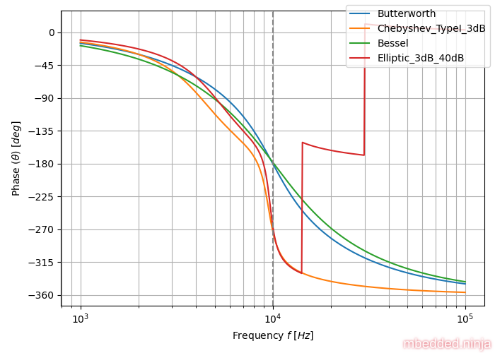
This is a placeholder for the reference: fig-tuning-comparison-phase-log shows the phase response of each filter tuning.

Phase comparison of different filter tunings.

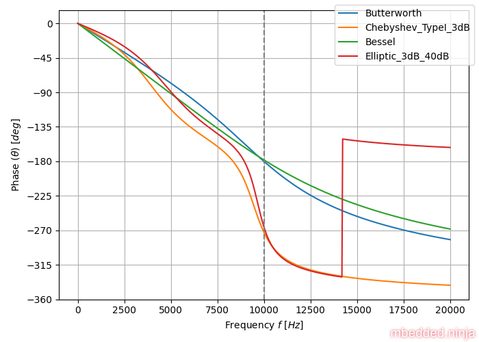
What you can’t easily pick out with logarithmic frequency axis is how linear the phase response is. So let’s replot the above but with a linear x-axis (frequency). We’ll stop plotting at twice the characteristic frequency.

Phase comparison of different filter tunings, with a linear x-axis (frequency) which makes it easy to see how linear the phase response is.

A comparison of group delay for the various filter tunings is shown in This is a placeholder for the reference: fig-tuning-comparison-group-delay. You can clearly shows the flat group delay of the Bessel filter, and the horrible response of the Chebyshev/Elliptic filter tunings.

Group delay comparison of different filter tunings.

The step response is also interesting to look at. The input step was from $0V$ to $1V$ and the output of each filter is shown in This is a placeholder for the reference: fig-tuning-comparison-step-response.

Step response comparison of different filter tunings.

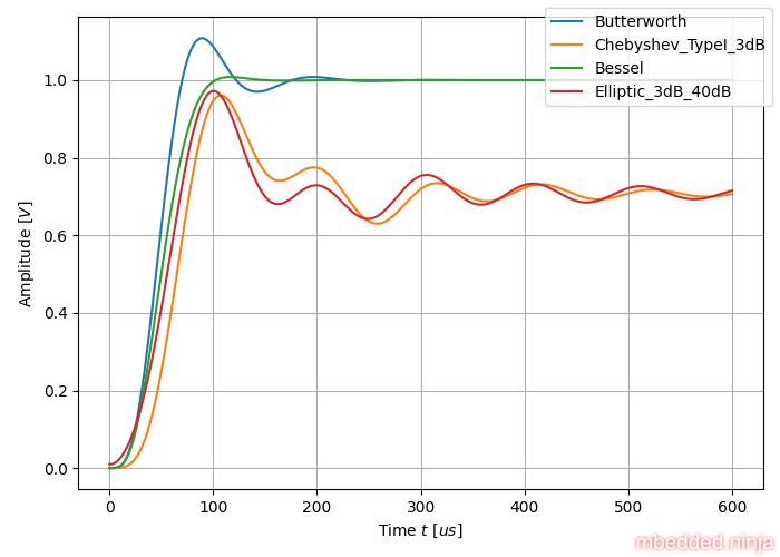
The Bessel-tuned filter shows the least amount of ringing. This is what we would expect, as the Bessel-filter is optimized to have the flattest group delay. All frequencies get delayed by roughly the same amount, and so the output is not “distorted”. Ringing is a result of different frequencies being delayed by different amounts of time (remember that an input step response essentially has frequency components at all frequencies, hence why it is a good testcase for a filter).

Further Reading

If you want to learn more about transfer functions, the Laplace transform, gain/phase plots and group delay, check out the What Are Transfer Functions, Poles, And Zeroes? page.

If you are interested in actually building a filter with these filter tunings, you’ll have to learn how to apply a specific filter tuning to a particular filter topology. For general filter topologies, see the Analog Filters page. For info specific to the popular 2nd-order Sallen-Key filter, see the Sallen-Key Filters page.

Footnotes

1. Wikipedia (2022, Aug 25). Butterworth Filter. Retrieved 2022-10-08, from https://en.wikipedia.org/wiki/Butterworth_filter. ↩ ↩²

2. Pieter P (2021, Jul 15). Butterworth Filters. Retrieved 2022-10-06, from https://tttapa.github.io/Pages/Mathematics/Systems-and-Control-Theory/Analog-Filters/Butterworth-Filters.html. ↩ ↩²

3. Wikipedia (2022, Oct 11). Chebyshev Filter. Retrieved 2022-10-14, from https://en.wikipedia.org/wiki/Chebyshev_filter. ↩

4. Wikipedia (2022, Oct 16). Chebyshev polynomials. Retrieved 2022-10-16, from https://en.wikipedia.org/wiki/Chebyshev_polynomials. ↩ ↩² ↩³

5. W. E. Thomson (1949, Nov). Delay networks having maximally flat frequency characteristics. 621.392.5: Paper No. 872 - Radio section. ↩

6. Wikipedia (2022, Oct 16). Bessel filter. Retrieved 2022-10-20, from https://en.wikipedia.org/wiki/Bessel_filter. ↩ ↩²

7. Sophocles J. Orfanidis (2006, Nov 20). Lecture Notes on Elliptic Filter Design. Rutgers University: Department of Electrical & Computer Engineering. Retrieved 2022-09-20, from https://www.ece.rutgers.edu/~orfanidi/ece521/notes.pdf. ↩ ↩²

8. Wikipedia (2022, Jan 30). Elliptic filter. Retrieved 2022-09-20, from https://en.wikipedia.org/wiki/Elliptic_filter. ↩ ↩²

9. Recording Blogs. Elliptic filter. Retrieved 2022-10-26, from https://www.recordingblogs.com/wiki/elliptic-filter. ↩