Electrical Noise

mbedded.ninja Author

Overview

Electrical noise is the unintentional (most of the time, but not in the case of stochastic resonance¹, dither, or random number generation) introduction of voltage/current disturbance in an electrical signal. Noise is added to a signal as it flows through a circuit/cable by the circuit components themselves, as well as being picked up by electromagnetic means from the surrounding environment. Noise is also emitted by a signal via electromagnetic means to the surrounding environment.

Noise on a power rail that was feeding 3 SMPS that hadn't been compensated correctly. Kept this image because I thought the waveform was interesting!

This page focuses on noise created by electronics components such as resistors, how to model it, and what it looks like. If you want to know how to protect your circuit from transient voltage spikes and other ESD events, see the ESD Protection page.

Noise Power Spectral Density (PSD)

The noise power spectral density (PSD) is a measure of the noise power per Hertz of bandwidth in a signal. It also called the noise spectral density, noise power density, or just noise density. Typically denoted with $N_0$ and has units $W / Hz$ . The $0$ in the symbol $N_0$ is used to distinguish a density (i.e., per $Hz$ ). Without the $0$ , $N$ represents a noise power over a specified bandwidth.

In the case that the noise power spectral density is constant (white noise), the noise power $N$ can be calculated from the noise power density $N_0$ with the following equation:

\begin{align} N = BN_0 \end{align}

where:
$N$ is the noise power, in Watts $W$
$B$ is the bandwidth of the signal, in Hertz $Hz$
$N_0$ is the white noise power spectral density, in $W / Hz$

Noise power spectral density can be either one-sided or double-sided. TODO: Add more info on this.

Noise Amplitude Spectral Density (ASD)

Noise amplitude spectral density (ASD) is an alternative to specifying a noise power spectral density. Instead of the noise power (in Watts), the noise "amplitude" is used. The amplitude is almost always either voltage or current (with voltage being the more common of the two). The symbol and units depend on whether voltage or current is used:

Noise voltage spectral density: Typical symbol $v_n$ and has units $V / \sqrt{HZ}$
Noise current spectral density: Typical symbol $i_n$ and has units $A / \sqrt{HZ}$

The noise voltage spectral density $v_n$ can be calculated from the noise power spectral density $N$ if you assume the load is a resistance of $1\Omega$ :

\begin{align} v_n = \sqrt{N} \end{align}

where:
$v_n$ is the noise voltage spectral density, in $V / \sqrt(Hz)$

Colours Of Noise (Power Law Noise)

The colour of noise refers to the shape of the power spectral density (PSD) with respect to the frequency. The category of noises that are assigned colours can also be called power law noise, as it's PSD is proportional to $\frac{1}{f^n}$ , where $n$ can be a positive (most commonly) or negative integer.

White noise: White noise is the simplest form of noise, and has a flat power spectral density when plotted against frequency (it has a spectral power density proportional to $1$ ).
Pink noise: Pink noise has a spectral power density proportional to $\frac{1}{f}$ .
Red noise: Red noise has a spectral power density proportional to $\frac{1}{f^2}$ . Also called Brownian noise.
Blue noise: Blue noise has a spectral power density proportional to $f$ .
Violet noise: Violet noise has a spectral power density proportional to $f^2$ .

If you don't have access to equipment that can perform a spectrum/frequency analysis on measured voltages or currents, you can roughly identify the "colour" of the noise sources by recognizing the "shape" of the noise in the time domain on a simple oscilloscope. The following sections contain examples of what each colour of noise looks like in both the time and frequency domain.

White Noise

White noise has a flat power spectral density when plotted against frequency. White noise got it's name from white light, which was assumed to have a flat power density spectrum across the visible range (the catch here is that, well, it actually doesn't). White noise can be specified by a single constant noise power spectral density value.

The following graph shows what Gaussian white noise looks like in the time domain:

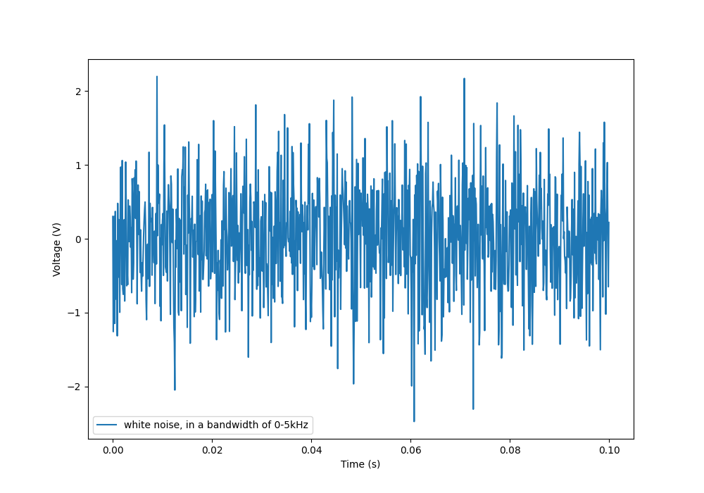
What white noise looks like in the time domain.

And this is what it looks like in the frequency domain (the discrete FFT of the above signal):

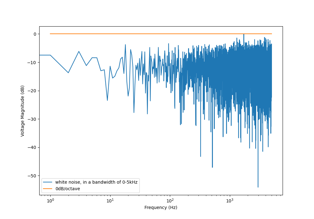
What white noise looks like in the frequency domain.

Although it commonly is modelled as such, white noise does not have to be Gaussian. Gaussian noise means the probability density function has a Gaussian distribution. However other forms of white noise exist, for example, Poisson white noise.

Examples of white noise include:

Thermal (Johnson-Nyquist) noise

Stochastic Resonance

Stochastic resonance is the clever technique of adding white noise to a signal which is usually too weak to be detected by the measurement device. The frequencies in the white noise which are also present in the signal will resonate with each other, amplifying the original signal but not amplifying the rest of the white noise. The system has to have a non-linear response for this to work¹.

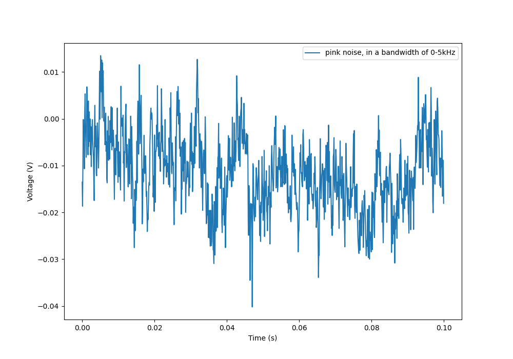
Pink Noise

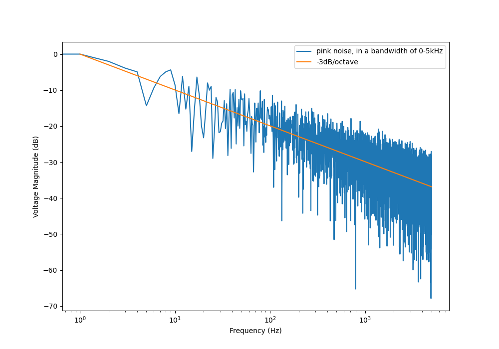
Also called $\frac{1}{f}$ noise. The PSD decreases at $3dB$ per octave.

The following graph shows what pink noise looks like in the time domain:

And this is what it looks like in the frequency domain (the discrete FFT of the above signal):

What pink noise looks like in the frequency domain.

Examples and uses of pink noise:

Interestingly, the frequency fluctuations of music have a $\frac{1}{f}$ spectral density. The reasoning behind this is that music generated by white‐noise sources sounded too random, while those generated by 1/f2 noise sounded too correlated². The "loudness" of music and speech also has a $\frac{1}{f}$ PSD.
The audio of steady rain fall or rustling leaves has a $\frac{1}{f}$ PSD.

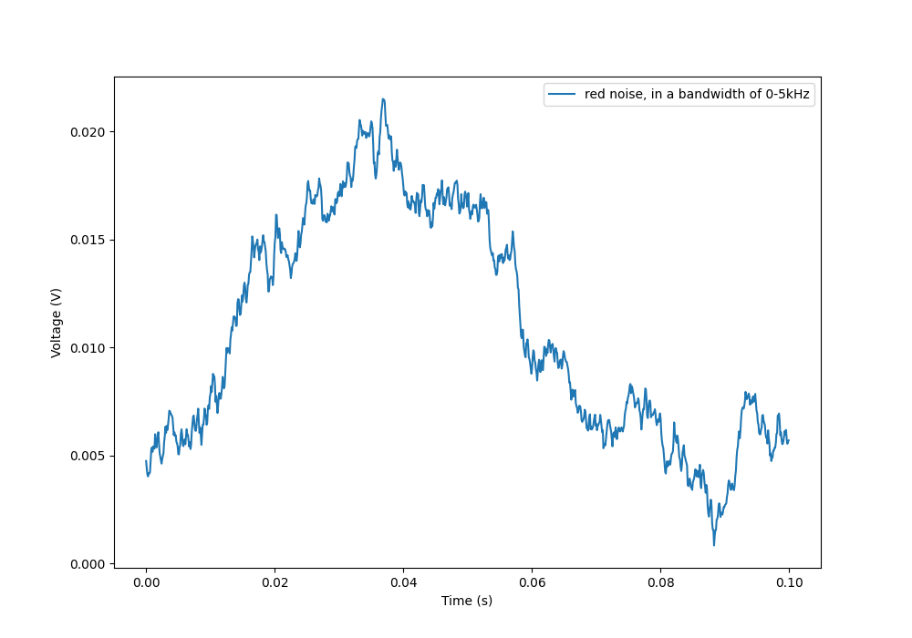
The following difference equation can create pink noise[^procaccia-schuster-universal-1-f-noise]:

\begin{align} x_t = (x_{t-1} + x_{t-1}^2)\ mod\ 1 \end{align}

Red (Brownian) Noise

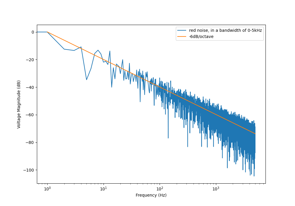
Also called Brownian or $\frac{1}{f^2}$ noise. The PSD decreases at $6dB$ per octave.

The following graph shows what red noise looks like in the time domain:

And this is what it looks like in the frequency domain (the discrete FFT of the above signal):

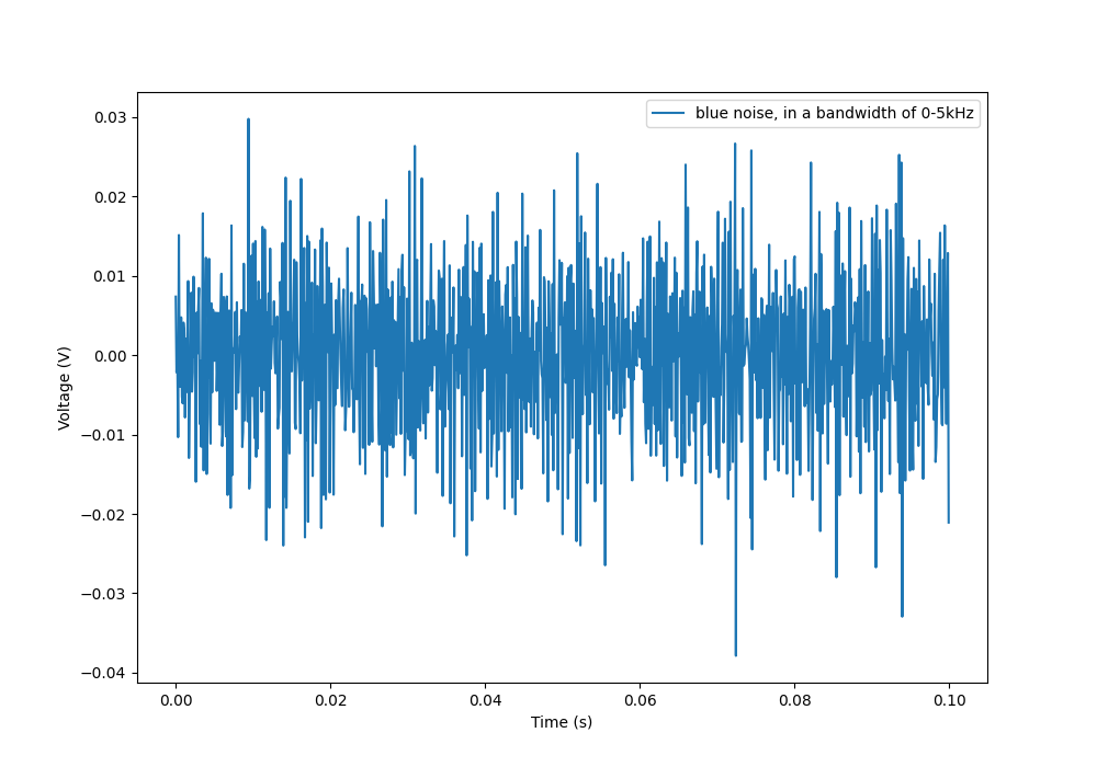
What red noise looks like in the frequency domain.

Blue Noise

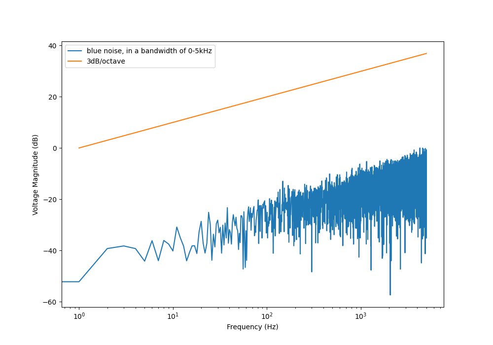
Also called Azure or $f$ noise. It has a PSD proportional to frequency. As the frequency goes up, the noise power goes up also. The PSD increases at $3dB$ per octave.

The following graph shows what blue noise looks like in the time domain:

And this is what it looks like in the frequency domain (the discrete FFT of the above signal):

What blue noise looks like in the frequency domain.

In the audio spectrum, blue noise sounds like a horrible high-pitched hiss.

Examples/uses of blue noise include:

Cherenkov radiation: A really interesting phenomenon which involves particles travelling faster than the speed of light (in a medium)!
Audio dithering: Blue noise can be added to audio tracks or imagery (a.k.a. spatial dithering of digital halftoning) to randomize the error in quantizing the digital signal³.

Non-Frequency Noise

Pops

Snaps

Crackles

So Where Does Electrical Noise Come From?

Thermal (Johnson-Nyquist) Noise

Thermal noise is generated in any resistor by the random movement of charge carriers (e.g. electrons in a typical circuit) due to them having thermal energy. It is also called Johnson, Nyquist or Johnson-Nyquist noise. Thermal noise increases with temperature, and for this reason some sensitive electronic circuitry is cooled down close to absolute zero to reduce the thermal noise in the sensor/instrument.

The noise power spectral density of thermal noise is found with the following equation:

\begin{align} N_0 = 4 k_B T R \end{align}

where:
$N_0$ is the one-sided noise power spectral density, in $WHz^{-1}$
$k_B$ is Boltzmann's constant, in $JK^{-1}$ ( $k_B = 1.380649\times10^{-23} JK^{-1}$ )
$T$ is the temperature of the resistor, in $K$
$R$ is the resistance of the resistor, in $\Omega$

This is commonly written as a voltage spectral density instead of power:

\begin{align} v_n &= \sqrt{N_0} \nonumber \\ \label{eq:thermal-noise-vsd} &= \sqrt{4 k_B T R} \end{align}

Example

For example, a $10k\Omega$ resistor at $25^{\circ}C$ has a noise power spectral density $N_0$ of:

\begin{align} N_0 &= 4 k_B T R \nonumber \\ &= 4 \cdot 1.380649\times10^{-23} JK^{-1} \cdot 298.15K \cdot 10k\Omega \nonumber \\ &= 1.647\times 10^{-16} W Hz^{-1} \nonumber \end{align}

Converting this to a noise voltage spectral density $v_n$ :

\begin{align} v_n &= \sqrt{N_0} \nonumber \\ &= \sqrt{1.647\times 10^{-16} W Hz^{-1}} \nonumber \\ &= 12.83 nV Hz^{-0.5} \end{align}

If our system had a bandwidth $B$ of $10kHz$ , then the RMS noise voltage would be:

\begin{align} v_{rms} &= v_n \cdot \sqrt{B} \nonumber \\ &= 12.83 nV / \sqrt{Hz} \cdot \sqrt{10kHz} \nonumber \\ &= 1.28uV \nonumber \end{align}

Instead of modelling the thermal noise source as a voltage in series with a noiseless resistor, you can model it as a current source in parallel with a noiseless resistor (the Norton equivalent). To get this equation, simply divide the thermal noise equation above in VSD by $R$ . This gives a current spectral density of:

\begin{align} i_n &= \frac{v_n}{R} \nonumber \\ &= \sqrt{\frac{4 k_B T}{R}} \end{align}

Shot Noise

Shot noise (a.k.a. Poisson noise) in electronic components arises from the random statistical fluctuations that occur in an electric current, due to electrical current not being a continuous flow but rather being made up of discrete (quantized) electrons travelling through a conductor. The PSD of Shot noise is independent of frequency, so it is spectrally [^_white_noise, white] (just like Thermal noise).

tip

Whilst shot noise can be considered white for practically all popular use cases, this assumption breaks down at really high frequencies and really low currents in where the frequency is now similar to the individual arrival rate of each electron (the law of large numbers no longer holds). This frequency is given by⁴:

\begin{align} f_0 &= \frac{I}{q} \end{align}

where:
$I$ is the average DC current, in Amps $A$
$q$ is the charge of an electron, in Coulombs $C$ ( $q = 1.602e^{-19} C$ )

Shot noise is typically talked about being present in semiconductor components such as diodes, and not in basic passives such as resistors. However, more recent literature suggests that shot noise is also present in basic resistors⁵.

The rms value of the shot noise current $i_n$ is given by the equation:

\begin{align} i_n &= \sqrt{2IqB} \end{align}

where:
$B$ is the bandwidth of the circuit/measurement, in Hertz $Hz$
and everything else as previously mentioned.

Current will create shot noise. When this current flows through a resistor, this will manifest itself as a noise voltage, in addition to the thermal noise of the resistor.

Example

A current of $1A$ measured over a bandwidth of $1kHz$ gives a RMS shot noise current value $i_n$ of:

\begin{align} i_n &= \sqrt{2IqB} \nonumber \\ &= \sqrt{2*1A*1.602e^{-19} C*1kHz} \nonumber \\ &= 17.9nA \nonumber \\ \end{align}

If this noise current is flowing through a resistor of $100\Omega$ , this will manifest in a noise voltage $v_n$ of:

\begin{align} v_n &= i_n R \nonumber \\ &= 17.9nA * 100\Omega \nonumber \\ &= 1.79uV \\ \end{align}

Shot noise also occurs in optics, such as photography, due to the discrete nature of the photons striking each pixel in the camera.

Addition of Noise Sources

The RMS amplitudes of independent noise sources add like orthogonal vectors (Pythagorean addition). If two independent voltage noise sources $v_{n1}$ and $v_{n2}$ were connected in series, then the total voltage noise $v_n$ is given by:

\begin{align} v_n^2 = v_{n1}^2 + v_{n2}^2 \end{align}

Noise sources like thermal noise and shot noise are independent.

Measuring Noise

Use the oscilloscope trigger for viewing the noise caused by specific aggressor events. Use the oscilloscope's infinite persistence measurement to measure total noise. It is good practice to measure of a time span of many minutes with the device operating in as many of it's different states as possible.

With the oscilloscope in averaging mode and it set up to trigger of a specific event, you can view the amount of noise due to that event. Any noise asynchronous to the event will be removed through repeated averaging.

RMS, dB, dBm, SD, Huh?

Noise measurements come in many different units. It can become very confusing when trying to compare different units or convert between them.

AC coupled waveforms become a little simpler...

For a waveform that has no DC component, the RMS value is the same as the standard deviation.

Typically, when doing noise measurements with an oscilloscope, AC coupling is turned on, which removes the DC component. This means that the standard deviation and the RMS measurements are equal.

Uncorrelated noise sources add in a root-sum-of-squares manner.

\begin{align} e_{total} = \sqrt{e_{1}^2 + e_{2}^2} \end{align}

This comes from the equation:

\begin{align} x_{rms}^2 = \bar{x}^2 + \sigma_{x}^2 \end{align}

where:
$x_{rms}$ is the RMS value of waveform x
$\bar{x}$ is the average (mean) of waveform x
$\sigma_{x}$ is the standard deviation of waveform x

As you can see, if the average of the waveform is 0 (as in the case when the waveform is AC coupled), the RMS value is the same as the standard deviation.

Creating Noise In Software

Power Law Noise

The following Python code is flexible enough to generate power law noise $\frac{1}{f^n}$ of any power $n$ . The code is from colorednoise.py, which uses an algorithm published by J. Timmer and M. Konig called On Generating Power Law Noise⁶. Depends on the popular Numpy library. This function was used to create the power law noise example signals on this page.

tip

You can also pass in negative exponents $-1$ , $-2$ to generate blue noise and purple noise.

from numpy import sqrt, newaxis
from numpy.fft import irfft, rfftfreq
from numpy.random import normal
from numpy import sum as npsum

def powerlaw_psd_gaussian(exponent, size, fmin=0):
    """
    Taken from https://github.com/felixpatzelt/colorednoise/blob/master/colorednoise.py
    Gaussian (1/f)**beta noise.
    Based on the algorithm in:
    Timmer, J. and Koenig, M.:
    On generating power law noise.
    Astron. Astrophys. 300, 707-710 (1995)
    Normalised to unit variance
    Parameters:
    -----------
    exponent : float
        The power-spectrum of the generated noise is proportional to
        S(f) = (1 / f)**beta
        flicker / pink noise:   exponent beta = 1
        brown noise:            exponent beta = 2
        Furthermore, the autocorrelation decays proportional to lag**-gamma
        with gamma = 1 - beta for 0 < beta < 1.
        There may be finite-size issues for beta close to one.
    shape : int or iterable
        The output has the given shape, and the desired power spectrum in
        the last coordinate. That is, the last dimension is taken as time,
        and all other components are independent.
    fmin : float, optional
        Low-frequency cutoff.
        Default: 0 corresponds to original paper. It is not actually
        zero, but 1/samples.
    Returns
    -------
    out : array
        The samples.
    Examples:
    ---------
    # generate 1/f noise == pink noise == flicker noise
    >>> import colorednoise as cn
    >>> y = cn.powerlaw_psd_gaussian(1, 5)
    """
    
    # Make sure size is a list so we can iterate it and assign to it.
    try:
        size = list(size)
    except TypeError:
        size = [size]
    
    # The number of samples in each time series
    samples = size[-1]
    
    # Calculate Frequencies (we assume a sample rate of one)
    # Use fft functions for real output (-> hermitian spectrum)
    f = rfftfreq(samples)
    
    # Build scaling factors for all frequencies
    s_scale = f
    fmin = max(fmin, 1./samples) # Low frequency cutoff
    ix   = npsum(s_scale < fmin)   # Index of the cutoff
    if ix and ix < len(s_scale):
        s_scale[:ix] = s_scale[ix]
    s_scale = s_scale**(-exponent/2.)
    
    # Calculate theoretical output standard deviation from scaling
    w      = s_scale[1:].copy()
    w[-1] *= (1 + (samples % 2)) / 2. # correct f = +-0.5
    sigma = 2 * sqrt(npsum(w**2)) / samples
    
    # Adjust size to generate one Fourier component per frequency
    size[-1] = len(f)

    # Add empty dimension(s) to broadcast s_scale along last
    # dimension of generated random power + phase (below)
    dims_to_add = len(size) - 1
    s_scale     = s_scale[(newaxis,) * dims_to_add + (Ellipsis,)]
    
    # Generate scaled random power + phase
    sr = normal(scale=s_scale, size=size)
    si = normal(scale=s_scale, size=size)
    
    # If the signal length is even, frequencies +/- 0.5 are equal
    # so the coefficient must be real.
    if not (samples % 2): si[...,-1] = 0
    
    # Regardless of signal length, the DC component must be real
    si[...,0] = 0
    
    # Combine power + corrected phase to Fourier components
    s  = sr + 1J * si
    
    # Transform to real time series & scale to unit variance
    y = irfft(s, n=samples, axis=-1) / sigma
    
    return y

Retrieved 2021-06-07, from https://en.wikipedia.org/wiki/Stochastic_resonance ↩ ↩²
Voss, R F, and Clarke, J. ''1/f noise'' in music: Music from 1/f noise. United States: N. p., 1978. Web. doi:10.1121/1.381721. ↩
Iliyan Georgiev and Marcos Fajardo: Blue-noise Dithered Sampling. https://www.arnoldrenderer.com/research/dither_abstract.pdf, accessed 2021-06-08. ↩
Imperial College. (2008). EE 3.02/A04 Instrumentation. Retrieved 2021-06-29, from http://cas.ee.ic.ac.uk/people/dario/files/E302/2-noise.pdf ↩
Marc de Jong. (1996, August). Sub-Poissonian shot noise. Nanophysics. Retrieved 2021-06-29, from https://www.lorentz.leidenuniv.nl/beenakker/beenakkr/mesoscopics/topics/noise/noise.html ↩
J. Timmer and M. Konig: On Generating Power Law Noise. Astronomy And Astrophysics 2.3.1995. Retrieved 2021-06-07, from https://citeseerx.ist.psu.edu/viewdoc/download?doi=10.1.1.29.5304&rep=rep1&type=pdf. ↩

Overview​

Noise Related Variables And Units​

Noise Power Spectral Density (PSD)​

Noise Amplitude Spectral Density (ASD)​

Colours Of Noise (Power Law Noise)​

White Noise​

Stochastic Resonance​

Pink Noise​

Red (Brownian) Noise​

Blue Noise​

Non-Frequency Noise​

Pops​

Snaps​

Crackles​

So Where Does Electrical Noise Come From?​

Thermal (Johnson-Nyquist) Noise​

Shot Noise​

Addition of Noise Sources​

Measuring Noise​

RMS, dB, dBm, SD, Huh?​

Creating Noise In Software​

Power Law Noise​

Footnotes​

Overview

Noise Related Variables And Units

Noise Power Spectral Density (PSD)

Noise Amplitude Spectral Density (ASD)

Colours Of Noise (Power Law Noise)

White Noise

Stochastic Resonance

Pink Noise

Red (Brownian) Noise

Blue Noise

Non-Frequency Noise

Pops

Snaps

Crackles

So Where Does Electrical Noise Come From?

Thermal (Johnson-Nyquist) Noise

Shot Noise

Addition of Noise Sources

Measuring Noise

RMS, dB, dBm, SD, Huh?

Creating Noise In Software

Power Law Noise

Footnotes