PID Control

PID control (a.k.a. three-term control¹) is a control technique using feedback that is very common in industrial applications. It is a good technique to use when you have a desired set-point for a process (system) to be in, and are able to control this with one variable. PID is an acronym for Proportional-Derivative-Integral, and describes the three mathematical processes used to calculate the output needed to control the process.

There are a few different PID topologies, including:

• Parallel form: Also known as ideal form or non-interacting. Easiest to understand, common in academia.
• Standard form: Coefficients have better intuitive meaning attached to them (and hence easier to tune), topology is common in industry.

These topologies are described in more detail in the following sections.

Common Terminology

No matter the topology, the goal of a PID controller is to control a process, given a single, measured process value ($y(t)$ or PV) that you want controlled (e.g. temperature of the heater) and a single variable you can adjust called the control value ($u(t)$ or CV) (e.g. voltage you can apply to the heaters coils). The output of the PID controller (which is the control value) is sometimes called $G(t)$.

The state you want to get the process to is called the set-point ($r(t)$ or SP). The set-point has the same units as the process value. The units of the control value is whatever is used to control the process.

Tip

I chose to use the variables $r(t), e(t), u(t), y(t)$ as used by Introduction: PID Controller Design ².

The error ($e(t)$) is always defined as the set-point minus the process value, so the error is positive when the actual value is less than what it needs to be. It is defined by the following equation:

$$\begin{align} e(t) = r(t) - y(t) \end{align}$$

where:
$e(t)$ is the error
$r(t)$ is the set-point (SP)
$y(t)$ is the process value (PV)
and everything else as previously mentioned

Example

Imagine a simple process in where you want to control the temperature of a room of your house by using an electric heater. You can vary the voltage to the heaters coils to vary the amount of thermal energy added to the room. You also have a thermometer to read the current room temperature. You want to keep the temperature of the room at a comfortable $22^{\circ}C$. The process variable $y(t)$ is the measured temperature of the room from the thermometer. The set point $r(t)$ is the desired $22^{\circ}C$. The control value $u$ is the voltage applied to the heating coils.

The error is $22^{\circ}C$ minus whatever the current measured temperature of the room is.

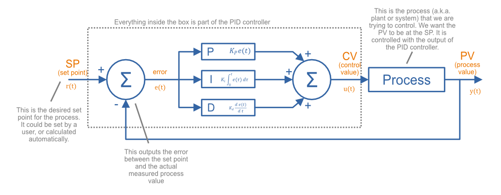
PID in Parallel Form

Inside a PID controller in parallel form (a.k.a. ideal form, non-interacting¹), the error is separately fed into the P (proportional), I (integral) and D (derivative) blocks of the PID controller. These blocks act on the error in different ways, and their output is summed together to generate the control value. The way these P, I and D blocks work is explained below.

This is called the parallel form because if you draw it as a block diagram, the proportional, integral and derivative terms all act in parallel to one another. The parallel form is easy to understand, but not so intuitive to tune³. Many academic related material will only mention this parallel form.

A block diagram of a PID controller.

The governing equation of a PID controller in parallel form is^{1 3}:

$$\begin{align} u(t) = K_{p}e(t) + K_{i}\int e(\tau) d\tau + K_{d}\frac{d}{dt}e(t) \end{align}$$

where:
$u(t)$ is the calculated control value (CV)
$e(t)$ is the error
$t$ is the current time
$\tau$ is the variable of integration (takes on values from time=0 to time=t)
$K_p$ is the proportional gain
$K_i$ is the integral gain
$K_d$ is the derivative gain

Tip

Notice that standard $t$ is used for the current time, and $\tau$ (tau) is used for the integration.

This can also be written in the Laplace domain as a transfer function¹:

$$\begin{align} G(s) &= K_p + \frac{K_i}{s} + K_{d}s \\ &= \frac{K_ds^2 + K_ps + K_i}{s} \\ \end{align}$$

This PID equation is in the continuous time domain. However, nowadays most PID control loops are implemented digitally. The discrete equation is written:

$$\begin{align} u(t) = K_{p}e_{k} + K_{i}T\sum\limits_{i=0}^k e_{k} + K_{d}\frac{(e_{k} - e_{k-1})}{T} \end{align}$$

where:
$T$ is the time period between samples

This equation is suitable for implementing in code. There also exists the Z transformation of the equation, but this obscures the physical meaning of the parameters used in the controller.

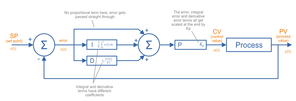
PID in Standard Form

A PID controller in standard form (a.k.a. ISA standard form^{4 5}) is more common in industry than in parallel form⁶. The factor $K_p$ is not just applied to the proportional term but instead brought out and applied at the end to all three factors (so it can be thought of as a scaling factor). Also, the factors that influence the integral and derivative terms now have better intuitive meaning.

Diagram of a PID controller in standard form.

The governing equation of a PID controller in standard form is¹:

$$\begin{align} u(t) = K_{p} \left( e(t) + \frac{1}{T_i}\int e(\tau) d\tau + T_d \frac{d}{dt}e(t) \right) \end{align}$$

where:
$T_i$ is the integral time
$T_d$ is the derivative time

The integral time $T_i$ refers to a scenario in where the error starts at 0, and then jumps to some fixed value. The proportional term will provide an immediate and fixed response, whilst the integral term will begin at 0 and slowly accumulate. The integral time is the amount of time it takes for the integral term to equal the proportional term.

The derivative time $T_d$ refers to a scenario where the error begins increasing at a fixed rate. The proportional term will start at 0 and begin to increase, whilst the derivative term will provide a fixed response. The derivative time is the amount of time for the proportional term to equal the derivative term.

Caution

Pay close attention to the fact that the integral term is multiplied by $\frac{1}{T_i}$ and not $T_i$. Unlike all other coefficients seen so far, this means that increasing $T_i$ does not strengthen the integral action, but weakens it. Also, you can never completely get rid of integral action when expressed this way, as for this $T_i$ would need to be $\infty$.

The parameters $K_i$ and $K_d$ in parallel form are related to the parameters $T_i$ and $T_d$ in standard form by:

$$\begin{align} K_i &= \frac{K_p}{T_i} \\ K_d &= K_p T_d \\ \end{align}$$

PID In Series Form

The governing equation of a PID controller in series form is⁷:

$$\begin{align} u(t) = K_{p} \left[ \left(\frac{T_d}{T_i} + 1\right) e(t) + \frac{1}{T_i}\int e(\tau) d\tau + T_d \frac{de(t)}{dt} \right] \end{align}$$

The proportional gain $K_d$ effects P, I and D actions just as with standard form, however the new difference is that with $\left(\frac{T_d}{T_i} + 1\right) e(t)$ the integral and derivative constants also affect the P action. This form is an artifact from the days of simpler, analogue and mechanical based PID controllers, in where the physical design of the controller was made easier if the equation was structured this way⁷. I have never seen this implemented on a new design with current digital technologies (e.g. microcontrollers and PLCs).

Gain vs. Bands

Some PID controllers work on absolute inputs and outputs (e.g. temperature in °C for the PV and SP, and power output to heater in Watts as the CV), whilst other PID controllers use inputs/outputs that represent the percentage of total range (i.e. their units are percent). One benefit of using percentages is that the PID loops can require less tuning adjustment when transferring to a different system, as the percentage-based inputs/outputs scale proportionally with the changing ranges of the system.

The band is also called the throttling range.

Commonly referred to as the throttling range (TR), proportional band is defined as the amount of change in the controlled variable required to drive the loop output from 0 to 100%.

$$\begin{align} PB = \frac{100}{G} \end{align}$$

For example, if the proportional band (PB) is 20%, then the proportional gain (G) is 5.

Tuning Methods

TODO: Add more tuning methods.

Manual Tuning

One method to perform manual tuning with a PID controller in parallel form is⁸:

1. Set the system to toggle slowly between two set points (with ample time between the changes to settle).

2. Set all gains to $0$.

3. Increase $K_p$ until the process continually oscillates in response to a disturbance.

4. Increase $K_d$ until the oscillations go away.

5. Repeat steps 3-4 until increasing $K_d$ does not make the oscillations go away.

6. Set $K_p$ and $K_d$ to the last known stable values.

7. Increase $K_i$ until it removes the steady-state error in an appropriate amount of time.

Example

Let’s go through an example manual tuning step with a mass-spring-damper (MSD) simulation. The MSD system has the following properties:

• $m=1kg$ (mass)
• $k=20Nm^{-1}$ (spring constant)
• $c=1Nsm^{-1}$ (damping constant)

The simulator time step is $1ms$. At $t=1s$, we change the set point from $0m$ to $1m$.

Let’s start of by setting all the gains to 0. As expected, we get no response:

1st step of tuning, set all gains to 0.

Now let’s increase $K_p$ until the system starts to oscillate continuously (increasing $K_p$ from left to right in the figure):

2st step of tuning, increasing $K_p$ until system continuously oscillates.

At $K_p=100$, we get continuous oscillation. Now increase $K_d$ until the oscillations are critically dampened:

3rd step of tuning, increasing $K_d$ until oscillations are dampened.

When $K_d=19$, the oscillations get critically dampened.

Repeat this process to see if we can still dampen the system. Let’s increase $K_p$ again until we get continuous oscillation:

4th step of tuning, increasing $K_p$ again.

At around $K_p=1800$ we start to get continuous oscillation. Can we dampen this by increasing $K_d$ again?

5th step of tuning, increasing $K_d$ to see if we can critically dampen the oscillations.

No we can’t! Somewhere between $K_d = 60{-}80$, rather than dampening the system further, we make the system unstable (see the right-most plot). Our loops of increasing $K_p$, $K_d$ are finished, and we go back to the last stable combination, which was $K_p=100$, $K_d=19$.

NOTE: We might be able to increase $K_p$ from $100$ to somewhere below $1800$ which can still be dampened, but for the purposes of this example we are going to say this is good enough and stop here.

Now the final step, increase $K_i$ until the steady-state error is eliminated in a suitable amount of time:

6th step of tuning, increasing $K_i$ until steady-state error is eliminated in a suitable amount of time.

At $K_i=200$, the system settles in about $1s$ with almost no steady-state error. So our final tuning parameters are:

• $K_p=100$
• $K_i=200$
• $K_d=19$

We get a little bit of overshoot, but this is fine for our application.

Integral Windup

Integral windup is a common problem with PID controllers. It is when a sudden change in the set-point or large disturbance on the output (really anything that causes a large error between where you are and where you want to be), causes the integral term to build up (remember that the integral term accumulates errors). Once you have reached where you want to be, the integral term has to “unwind”, and will drive the output past the setpoint until the error-time product is unwound.

Ways of preventing integral windup:

Limit Integral Effort To Fixed Values

This is the simplest form of preventing integral windup. Windup is preventing by limiting the integral effort to fixed maximum/minimum values. If the integral efforts begins to exceed the set max/min values, it is limited to these max/min values. Note that the integral effort is not reset. This is a common point of confusion, as sometimes the process of preventing integral windup is called “resetting”.

Limit Integral Effort Based On Output Limits

If output limits exist (they should for most real-world processes), the integral effort can be limited when the output hits it’s limits.

For example, say the P, I and D terms were contributing the following effort to the output:

• P = 6
• I = 5
• D = 2

Lets pretend the output is limited to 10. P + I + D = 13, so the output is going to be saturated. The I effort is likely to be even larger next iteration (assuming we haven’t reached our set-point yet) and so the output will saturate even more. To prevent this, we could limit the I value so that the sum of all three just hits the saturation limit, e.g. I would be set to 2.

Be careful not to set the integral term to a negative value! This could potentially occur if the P + D term were already larger than the saturated value.

Getting Rid Of Derivative Kick

Derivative Kick is the name for large output (CV) swings when a step-change in the set point (SP) occurs. When the set point changes abruptedly (you want the temperature of the room to be 20°C, but now someone else has come along and set it 25°C), the derivative of error is mathematically infinite! In a discrete, sampled based system this essentially results in a really large number. Remembering that the derivative term is:

$$\begin{align} \text{derivative term} = K_{d}\frac{d}{dt}e(t) \end{align}$$

this results in a huge spike (kick) in the output (CV). Luckily, when implementing a PID controller, there is an easy way to fix this. Remember that the error is:

$$\begin{align} e(t) = SP - PV \end{align}$$

If we take the derivative of this:

$$\begin{align} \frac{d}{dt}e(t) = \frac{d}{dt}(SP - PV) \end{align}$$

The trick is to now assume the SP is constant. If the SP is constant, then the derivative of a constant is just 0. Thus:

$$\begin{align} \frac{d}{dt}e(t) = -\frac{d}{dt}(PV) \end{align}$$

So for the derivative term, rather than calculating the change in error as the change in SP - PV, we just use the negative change in PV. In code, this would look like:

delta_error = new_error - last_error # Don't do this, results in derivative kick
delta_error = new_PV - last_PV # Do this instead! No derivative kick with change in set pint!
d_term = delta_error / delta_time

This gets rid of derivative kick in the PID controller when the set point changes abruptedly.

Feedforward

In the context of PID control, feedforward is the act of computing a best guess at the needed control value from measured process variables, and using this information to assist the PID control. Generally you are making predictions on what the control value will need to be based of physical laws and knowledge of how the system works. PID without feedforward does not predict what is going to happen before it happens --- it only operates on the error once it has occurred. Feedforward can help by providing some prediction of what is going to happen, before it happens (proactively)⁹.

A PID controller with feedforward added.

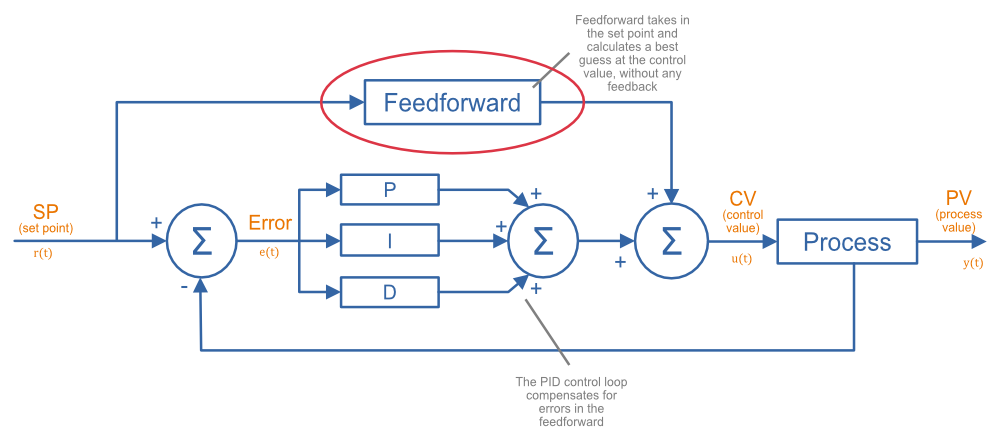
In typical PID controllers with feedforward, a large proportion of the control value is actually generated by the feedforward, and only a small amount by the PID loop, which aims to correct for any inaccuracies in the feedforward model of the system.

Example

Imagine a basic PID controller which wants to set the voltage across the fixed resistor (with known resistance). It is able to measure the voltage across the resistor and change this voltage by changing the current (i.e. the output of the PID controller is connected to a current source). A primitive PID loop would accept a set point, and then change the current based on the error between the set point and process value.

A PID controller with feedforward might improve on this by realizing that we can calculate the current needed to get to the set point based on Ohm’s law, i.e. $I = \frac{V}{R}$. This feedforward will give us most of the required control value, but we still want to keep the PID loop to modify the control value slightly to fix any inaccuracies, e.g. measurement error in the resistance or accuracy of the current source.

Feedforward control can be difficult to implement when the process behaviour is not well understood, or it’s hard to measure the variables which disturb the process. In many cases, when basic PID control alone is sufficient, adding feedforward is not worth the extra complexity.

Worked Example Using The Parallel Form

Lets assume a mass/spring/damper process (aka plant or system) which consists of a mass attached to a fixed wall by spring and damper. We want to control the position of the mass, relative to it’s resting point (which will be when the spring exerts no force). We can control the mass by applying an external force to the mass, $F_{ext}$.

A mass-spring-damper system, which is commonly used to demonstrate PID control and appropriate tuning.

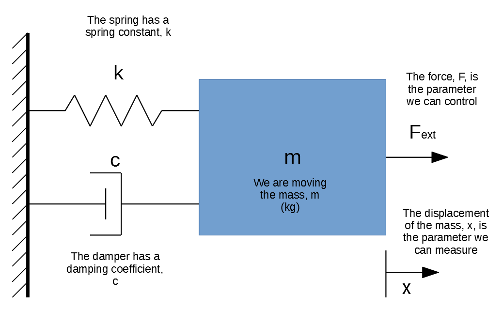
The Physics

The mass $m$ is $2kg$. The spring has a spring constant, $k$, which is $5Nm^{-1}$. The damping coefficient $c$ is $3 Nsm^{-1}$.

We can model the system using Newton’s equation:

$F = ma$

Summing up the forces on the mass $m$ gives:

$F_{ext} - F_{spring} - F_{damper} = m\ddot{x}$

Substituting in the equations for the spring and damper give:

$F_{ext} - kx - c\dot{x} = m\ddot{x}$

where:
$x$ is the displacement
$\dot{x}$ is the first derivative of $x$ (i.e. velocity)
$\ddot{x}$ is the second derivative of $x$ (i.e. acceleration)

We can simulate this system in code by discretizing the system into small time steps, and assume linear values for the acceleration and velocity over these small time steps.

How The Simulation Works

1. Assume starting conditions of displacement, velocity and acceleration are 0. $F_{ext}$ is the control variable (set by the PID controller).

2. Determine a suitably small time step, $\Delta{T}$. Then for each time step:

3. Calculate the force exerted by the spring and damper.

   $F_{spring} = kx$

   $F_{damper} = c\dot{x}$

4. Determine the output of the PID controller $F_{ext}$, providing it the setpoint and “measured” displacement (which starts at 0, and then gets re-calculated at each time step as below).

5. Calculate the acceleration for this time step:

   $\ddot{x} = \frac{F_{ext} - F_{spring} - F_{damper}}{m}$

6. Calculate the change in velocity and displacement for this time step:

   $\Delta{\dot{x}} = \ddot{x} \Delta{T}$

   $\Delta{x} = \dot{x} \Delta{T}$

   Note that these are changes in velocity and displacement, so to calculate the current velocity and displacement you add this change to the stored velocity/displacement state.

7. Once the values for the velocity and displacement are updated, repeat steps 3-5 for the next time step. $F_{spring}$ and $F_{damper}$ will calculated for the next time step using these updated velocity and displacement values.

Running The Simulation

We’ll apply a step change at $t=1s$, changing the setpoint to $r(t) = 1m$. We’ll use a time step of $\Delta{T}=10ms$. We’ll use the parallel form of PID controller:

$$\begin{align} u(t) = K_{p}e(t) + K_{i}\int e(\tau) d\tau + K_{d}\frac{d}{dt}e(t) \end{align}$$

Let’s begin by just adding some proportional gain. Let’s set $K_p=10, K_i=0, K_d=0$:

The response of the mass-spring-damper system with just proportional gain.

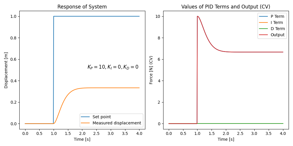
You can clearly see that this PID controller does not work very well. It only moves the block to about $0.3m$ and then stops. Let’s bump up the proportional gain to see if we can reduce the error further:

The response of the mass-spring-damper system with more proportional gain.

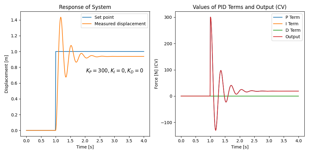
It’s better, but we still have significant steady-state error, and we’ve now got overshoot. Steady-state error is almost unavoidable with only pure proportional control. Integral control is perfect at fixing steady-state error, so let’s add some. We’ll fix the overshoot later:

The response of the mass-spring-damper system with more proportional gain.

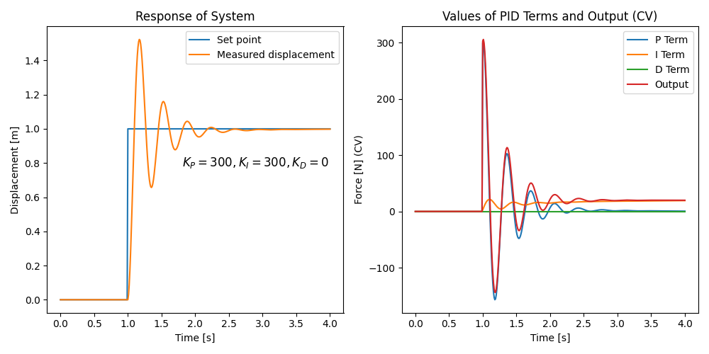
Getting better! You can see the effect of adding the integral control, the steady state error is now eventually removed. Now let’s see if we can get rid of the overshoot by adding some derivative control:

The response of the mass-spring-damper system with derivative control added.

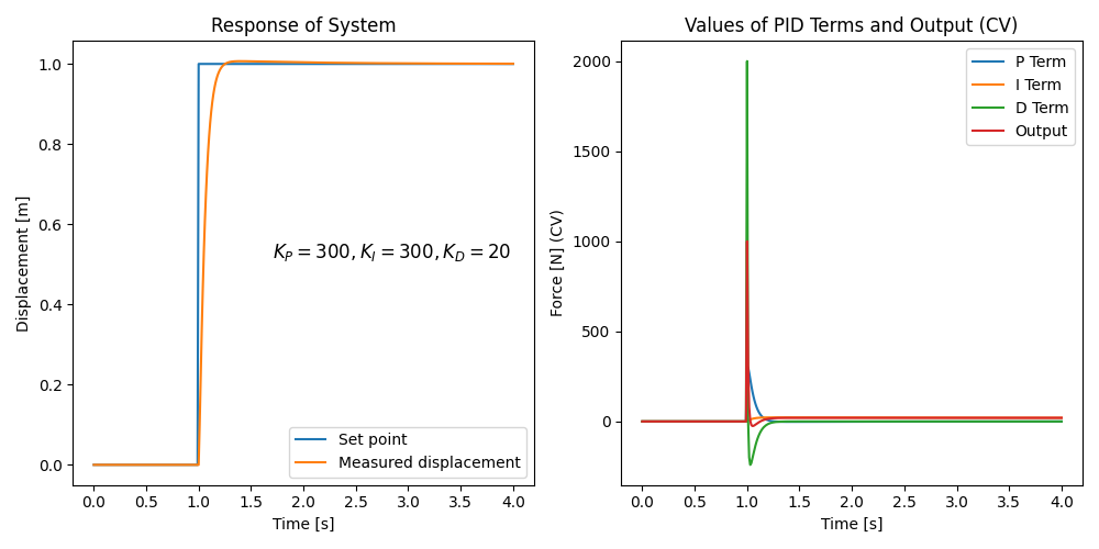
Now we are looking pretty good! We’ve completely removed the oscillations at the process reaches the setpoint pretty quickly. Note though that the derivative terms introduces a huge “kick” when the step change happens (this makes sense, because at that point there is a huge change in error!). This may saturate the actual thing connected to the control output (e.g. a linear motor which provides the external force), and control value limiting may need to be added to the PID controller.

Tip

I’m not claiming to have just stumbled across coefficients that seemed to work well, to get to these values I spent a bit of time experimenting with the numbers. I didn’t follow any specific tuning method.

If you are interested in the Python code that was used to perform this simulation, see here.

Firmware Modules

If you are looking for PID code for an embedded system, check out my Pid project on GitHub (CP3id). It is written in C++ and designed to be portable enough to run on many embedded systems, as well as Linux.

More Resources

Improving The Beginners PID: Introduction is a great set of articles explaining PID control loops and use Arduino code examples to supplement the explanations.

Practical Process Control: Proven Methods And Best Practices For Automated Process Control has lots of useful information on PID.

Implementing PID Controllers with Python Yield Statement has some interesting examples on using the yield statement in Python to help create a PID controller.

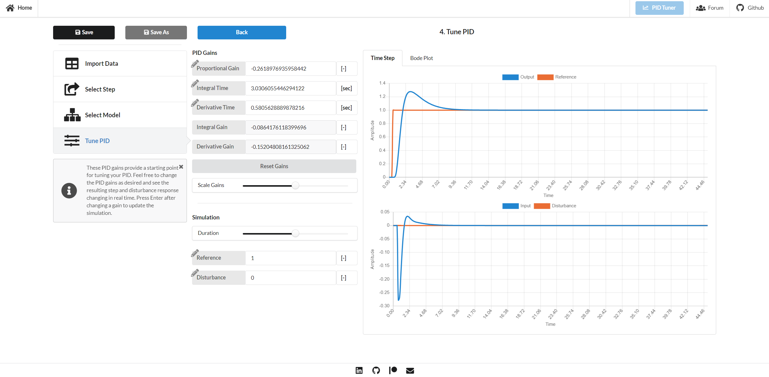
pidtuner.com is a free, open-source PID tuning web application. It works by allowing you to import measured output/input data, then select a single step change within the data, apply a mathematical model to the system, and then play around with P, I and D coefficients and see how the system responds¹⁰.

Screenshot of the PID tuning app at pidtuner.com¹⁰.

References

Footnotes

1. Wikipedia (2022, Mar 30). PID controller. Retrieved 2022-05-07, from https://en.wikipedia.org/wiki/PID_controller. ↩ ↩² ↩³ ↩⁴ ↩⁵

2. University of Michigan - Control Tutorials For MATLAB and SIMULINK. Introduction: PID Controller Design. Retrieved 2023-06-24, from https://ctms.engin.umich.edu/CTMS/index.php?example=Introduction&section=ControlPID. ↩

3. Jacques Smuts (2010, Mar 30). PID Controller Algorithms [Blog Post]. Retrieved 2023-06-23, from https://blog.opticontrols.com/archives/124. ↩ ↩²

4. Control (2014, Oct 27). PID Form Trick or Treat Tips [Blog Post]. Retrieved 2023-06-23, from https://www.controlglobal.com/home/blog/11328993/pid-form-trick-or-treat-tips. ↩

5. Vance Vandoren (2016, Jul 26). Understanding PID control and loop tuning fundamentals [Web Page]. Control Engineering. Retrieved 2023-06-23, from https://www.controleng.com/articles/understanding-pid-control-and-loop-tuning-fundamentals/. ↩

6. Wilderness Labs. Standard PID Algorithm - Understanding the real-world PID algorithm [Web Page]. Retrieved 2023-06-23, from http://developer.wildernesslabs.co/Hardware/Reference/Algorithms/Proportional_Integral_Derivative/Standard_PID_Algorithm/. ↩

7. Tony R. Kuphaldt. PID Controllers : Parallel, Ideal & Series [Web Page]. Instrumentation Tools. Retrieved 2023-06-24, from https://instrumentationtools.com/pid-controllers/. ↩ ↩²

8. hauptmech (2012, Oct 27). What are good strategies for tuning PID loops? [Forum Post]. Stack Exchange - Robotics. Retrieved 2023-06-24, from https://robotics.stackexchange.com/questions/167/what-are-good-strategies-for-tuning-pid-loops. ↩

9. Pramit Patodi (2020, Jul 14). Benefits in feedforward in PID controllers [Blog Post]. IncaTools. Retrieved 2023-06-22, from http://blog.incatools.com/benefits-feedforward-pid-controllers. ↩

10. pidtuner.com. Tune your PID - It has never been easier [Web Page]. Retrieved 2023-06-27, from https://pidtuner.com/#/. ↩ ↩²