CRCs (Cyclic Redundancy Checks)

CRCs (Cyclic Redundancy Checks) are a type of checksum that is used to detect errors in data transmission. It is based on modulo-2 polynomial (GF(2)) division.
“Everything you wanted to know about CRC algorithms, but were afraid to ask for fear that errors in your understanding might be detected.” - Ross N. Williams.1
How They Work
The general idea behind a CRC is to treat the input data as one huge number, divide it by another fixed number, and make the remainder from this division the checksum. It turns out that division (as long as the divisor is about as big as the checksum) is good at creating “chaos” in the checksum, meaning that small changes in the input data will result in a large change in the checksum.
Imagine the data [0x05, 0xB8]. Pretend our divider is 0x05. We can treat the data as the single number 0x05B8 (concatenating the bytes together). We can then divide 0x05B8 by 0x05 and get a remainder of 0x04. This is our checksum. This is obviously easy to do with simple CPU arithmetic when the data is just two bytes. However, when the data is much larger, it becomes more difficult to do this in a single operation. Instead, we can use long division to “iterate” through the data one bit at a time.
Doing it the long division way on our data [0x05, 0xB8] with our divider 0x05 would look like this:
0b100100100 _____________0b101 ) 0b10110111000 0b10100000000 (0b101 << 8 = 1280) ------------- 0b00010111000 (= 184) 0b00010100000 (0b101 << 5 = 160) ------------- 0b00000011000 (= 24) 0b00000010100 (0b101 << 2 = 20, also note a borrow happens here) ------------- 0b00000000100 (= 4 = remainder)Instead of the numbers being treated as positive integers, CRCs treat them as polynomials (this includes the dividend (data), divisor, and remainder). This is done by treating the bit string whose bits are the coefficients of the polynomial. For example, our divisor of 0xFA is 0b11111010, which in polynomial form is which simplifies to .
But how does division work with polynomials rather than numbers? This is where it gets a bit weird, and the field (Galois field of two elements) comes into play. The rule is decided that the polynomial arithmetic will be all modulo 2. This is essentially the same as binary arithmetic with no carry.
Addition and Subtraction
Addition without carry is the same as XOR. For example:
1001+1010----- 0011Subtraction is the same as addition.
Multiplication
For multiplication, the cleanest way to see what’s going on is to do it on the polynomials first. As an example, 1011 is and 1010 is . Multiplying them out the ordinary way:
The term has a coefficient of 2, but coefficients live in GF(2) where , so that whole term vanishes:
Reading off the coefficients gives the bit string 1001110.
Doing the same thing directly on the binary representation, multiplication becomes “for every set bit at position in the multiplier, XOR a copy of the multiplicand shifted left by .” Laid out as long multiplication:
1011 x 1010 ------ 0000 (bit 0 of 1010 = 0) 1011 (bit 1 of 1010 = 1, shifted left 1) 0000 (bit 2 of 1010 = 0)1011 (bit 3 of 1010 = 1, shifted left 3)-------1021110 (column-wise sums — the 2 at bit position 4 is the same 2 as in the $2x^4$ coefficient above)1001110 (after mod 2 collapses the 2 to 0)The column-overlap at bit position 4 (where the shift-by-1 and shift-by-3 partials both contribute a 1) is exactly the source of the term in the polynomial form. The mod-2 rule kills it in either representation, so the two methods agree on the final answer 1001110.
Division
Now let’s explore division. We’ll do it as polynomials first, then binary. As a small example, let’s divide 1101001 by 1001 — that is, by .
In polynomial form, long division works just like ordinary algebra. The leading term of the quotient is whatever cancels the leading term of the dividend.
Step 1: , so the first quotient term is . Multiply back: . Subtract from the dividend:
Remember that subtraction in GF(2) is the same as addition, so the and terms each cancel against their counterparts.
Step 2: , so the next quotient term is . Multiply: . Subtract:
The remainder has degree 2, less than the divisor’s degree 3, so we are done. The quotient is and the remainder is .
In binary, the same idea works directly with bit-shifts and XORs. Here’s 1101001 ÷ 1001 laid out in the standard long-division form:
1100 (quotient) ________1001 ) 1101001 (divider | dividend) 1001 ------- 100001 1001 ------ 00101 0000 ----, 0101 0000 ---- 101 (remainder)What is happening above? At each step, look at the leftmost bit of the working window: if it’s 1, we subtract the divisor from the dividend by XORing in the divisor (1001); if it’s 0, XOR in 0000 instead (a no-op kept for layout regularity — see iterations 3 and 4, which are the bit-by-bit version’s way of saying “the polynomial division would have already stopped”). Then shift the window one column to the right, bringing in the next bit of the dividend.
In future examples we will skip all the no-op XOR with 0000 steps for brevity. And we also skip writing down the quotient — no one cares about this in CRC calculations.
The quotient 1100 () and remainder 101 () match the polynomial result above. For CRC purposes the quotient is discarded — only the remainder matters. Taking the remainder of polynomial division is exactly how a CRC is computed. The dividend is the message with zero bits appended (where is the degree of the generator polynomial), and the divisor is the generator.
The Generator Polynomial
Now that we have a basic understanding of CRC maths, what is the generator polynomial? This is the polynomial that is used to divide the data by. For example, it could be . It is commonly represented as a hexadecimal number rather than as a traditional polynomial. A really important point to note is that the leading one is dropped from the hex representation by convention. For example:
- Polynomial:
- Binary:
0b1011 - Hex:
0x3(leading one is dropped!)
The width of the polynomial is the position of the leading bit, counting from 0. So the width of the polynomial 0b1011 is 3, not 4. This is one of the most important parts of the polynomial, as it determines the width of the CRC value. This is because the remainder (CRC value) will always be less than the divisor (this should be any obvious truth about any division).
You could choose any polynomial, but some are better than others at detecting errors. The science behind choosing a polynomial is a bit of a dark art, and generally you are advised to pick a standard and use that rather than coming up with your own!
Calculating the CRC is now done by:
- Appending zero bits to the data, where is the width of the generator polynomial.
- Dividing the data by the generator polynomial to work out the remainder. This is the CRC value!
Next, the CRC value is appended to the data (taking the place of those zero bits we appended earlier). So we would send the following to the receiver:
11010011011 (data + crc)When the receiver gets the data, it needs to check if the message is valid. To do this, it could split the message into the original data and the CRC value and do the same CRC calculation on the original data. If the calculated CRC value matches the CRC value embedded in the message then the message is valid. However, there is a trick which makes things simpler. Rather than splitting the message up, the receiver can just calculate the CRC of the entire message (including the CRC value embedded into it by the sender). If the calculated CRC value is 0, the message is valid. Why does this work? This is because we added the remainder onto the data. Remember in arithmetic, addition is the same as subtraction. So it’s the same as subtracting the remainder from the data. If you subtract the remainder, you are left with a number which perfectly divides by the polynomial and gives 0 remainder, hence a CRC value of 0.
Choosing a Polynomial
So before we talked about how once we add the remainder to the original data, the message is perfectly divisible by the polynomial. This means the transmitted message is a integer multiple of the polynomial .
If the message is corrupted during transmission, then the received message will be:
where is the error pattern and is CRC addition (XOR). The receiver divides by . We know that (mod is the same thing as remainder):
So thus:
Any corruption that just so happens to make a multiple of will go undetected by the receiver. So we want to choose a polynomial whose multiples are not anything like the kind of error patterns we are likely to see during transmission.
Single Bit Errors
Single bit errors are where would be things like 1000, 0100, 0010, and 0001. This means a single bit has been flipped in the message. In polynomial form this would be where is an integer. These are easy to detect, as we just need to make sure that has at least two bits set to 1. Any non-zero multiple of will also have at least two bits set to 1, and thus will never divide evenly.
For example, if was 101, then in polynomial form . There is no way to divide by and leave no remainder as the only things that divide cleanly are where .
Two Bit Errors
This is where the maths and logic starts to get more involved, and I don’t understand exactly how it works. But there are ways to design the polynomial so that it can detect all two bit errors.
Error With an Odd Number of Bits
All errors with an odd numbers of bits can be detected by making sure the polynomial has an even number of bits set to 1. This is because:
- Multiplication in GF(2) is XORing the polynomial bits and various shifted positions against the data.
- XORing a number with an even number of bits (the polynomial) preserves the “oddness” property of the number.
Burst Errors
All burst errors up to a certain length can be detected by making sure the polynomial has its lowest bit set to 1.1
Summary
There is no one “best” polynomial to choose. There are certainly some that are bad choices and there are some which a better choices for certain applications. There are “best” polynomials with regards to specific Hamming distance properties, but these assume the data is affected by low, constant, random, independent bit errors.3 This is usually not the case in practice, bit errors tend to occur in bursts and may affect a sequence of bits all in the same direction.
Implementing a CRC Algorithm in Software
The key things we have to do is CRC division. We can’t just use the normal division instruction all CPUs have since:
- We are using mod 2 arithmetic (a.k.a. GF(2), CRC arithmetic), not regular division.
- The number we are dividing is the entire message, which could be many bytes, kBs, MBs long. Most CPUs/standard libraries/compilers only support numbers up to 8 or 16 bytes (64 or 128 bits).
So we have to implement our own CRC division algorithm. The simplest way is to repeat in code the long division algorithm we used above. We can do this by:
- Creating a variable which represents the in-progress remainder. The variable’s width is the degree of the generator polynomial — i.e. one less than the polynomial’s bit-width. For polynomial
1011(4 bits, degree 3), the variable is 3 bits, starting at000. - Shift the variable left by 1 bit. On the low end, shift in the next bit of the augmented message (the message with the zero bits appended). The MSB of the message is taken first (i.e. the topmost bit of the highest byte). The bit that falls off the high end of the variable is the “popped” bit.
- If the popped bit was a 1, XOR the variable with the generator polynomial minus its leading 1 (the same form discussed earlier — for
1011, that’s011).
This method is essentially the same as the CRC hardware implementation using a LFSR (Linear Feedback Shift Register).
A Faster Software Implementation
The above implementation is basic, but slow. It has to iterate over every bit in the message individually. To speed this up, we ideally want a way of operating on bytes (or multiple bytes) at a time. This is possible by using the “table” method. For the purposes of an example, let’s assume we are using a CRC polynomial with a width of 32 bits (4 bytes).
Now our register will be 32 bits wide as shown in the diagram below.
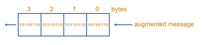
Let’s assume the top byte 3 has register values:
r7 r6 r5 r4 r3 r2 r1 r0In the next iteration, r7 will determine whether the poly is XORed into the entire register. If r7 is 1, then the poly is XORed into the entire register. If the top 8 bits of the poly are p7 p6 p5 p4 p3 p2 p1 p0, then the register will have this value:
r6 r5 r4 r3 r2 r1 r0 ??+ r7 * (p7 p6 p5 p4 p3 p2 p1 p0)Where + is XOR and * is multiplication (the multiplication makes sure the poly is only XORed if r7 is 1, otherwise it’s just an XOR with all 0’s, i.e. a no-op).
The new top bit, which controls what happens in the next iteration, is now r6 + r7 * p7. Generalising: after 8 shift-and-XOR iterations, every bit in the register is some fixed XOR combination of the original 8 top bits and the (constant) poly bits. The poly never changes, so the only input to that 8-iteration result is the top byte of the register. With possible top-byte values, we can precompute the answer for every one of them and store the results in a 256-entry table of 32-bit XOR masks.
To build the table: for each from 0 to 255, load the register with in the top byte, run the bit-by-bit algorithm for 8 iterations, and store the resulting register value as table[i].
Now the inner loop processes one byte per iteration. Here is Python pseudo-code for the calculation:
while augmented_msg_bytes_remaining: top_byte = register >> 24 # Extract top byte register = (register << 8) & 0xFFFFFFFF # Shift up by one byte register |= next_augmented_msg_byte # Bring new byte in at bottom register ^= table[top_byte] # Apply precomputed XORThis is roughly 8x faster than the bit-by-bit version. Variants like slice-by-4 and slice-by-8 use multiple tables in parallel for further speedups, and modern x86 (SSE4.2 CRC32 instruction) and ARM64 hardware-accelerate this further.
Initial Values
So far we have been assuming that the initial value of the CRC residual variable is initialized to 0. This is not always the case. Many CRC algorithms start with a non-zero initial value. Why? There is quite a problem with CRC algorithms that start with all 0s - the CRC value does not change with any leading zero bits, and thus cannot detect errors if 0 bits are missing/added. This type of error can be quite common in practise, and many CRC algorithm start with a non-zero init value to compensate. I would always prefer to select an algorithm with a non-zero init value unless there is a very good reason to use a 0 init value.
The most popular non-zero initial value is just all f’s, e.g. 0xffff for a 16-bit CRC.
CRC Calculator
Use the calculator below to compute the CRC of arbitrary data against any of 40 pre-defined CRC algorithms — from CRC-3/ROHC up to CRC-64. Switch between ASCII / UTF-8 and hex input via the Format radio buttons. Expand “Algorithm parameters” to see the polynomial, init / XOR-out values and check value for the selected algorithm.
Algorithm parameters
| Width | 32 bits |
|---|---|
| Polynomial | 0x04C11DB7 |
| Initial value | 0xFFFFFFFF |
| Reflect data | Yes |
| Reflect remainder | Yes |
| Final XOR | 0xFFFFFFFF |
| Check value (CRC of "123456789") | 0xCBF43926 |
Processor Support
Some processors have dedicated instructions for CRC calculations. Some Intel processors have the SSE4.2 instruction set (Streaming SIMD Extensions 4.2) which includes the CRC32 instruction. This was first introduced in the Nehalem microarchitecture.4 This accumulates a CRC32C (Castagnoli) value using the polynomial 0x1EDC6F41.5 AArch64 architecture provides hardware acceleration for the CRC-32 and CRC-32C algorithms.4
Some Common CRC Algorithms
Note that this does in no way try and be an exhaustive list. Sites like CRC RevEng - Catalogue of parameterized CRC algorithms and Prof. Koopman’s CRC Polynomial Zoo have great detailed lists of CRC algorithms.
The following algorithms are parameterized following the convention used by Dr Ross Williams in his A Painless Guide To CRC Error Detection Algorithms paper:1
- Name: The name of the CRC algorithm. We use the name specified by Ross Williams if possible.
- Width: The width of the CRC in bits. This is always the same as the degree of the polynomial.
- Poly: The polynomial of the CRC algorithm, expressed as a hexadecimal number. The leading one (the coefficient of the highest power of ) is dropped from the hex value.
- Init: The initial value of the CRC algorithm before any input data is processed.
- RefIn: Whether the input is reflected (bits are swapped around their center, e.g.
11001010reflected becomes01010011). Iffalse, input bytes are treated as bit 7 being the most significant bit and bit 0 being the least significant bit. Iftruethe input is reflected first so that all the bits are reversed in order. - RefOut: Whether the output is reflected. If
false, the output is fed directly into the XOR function after running through input data. Iftrue, the output is reflected first so that all the bits are reversed in order (similar to RefIn). - XorOut: This is the value that the result is finally XORed with before being returned as the final CRC value. This affects the residue and can make it non-zero.
- Check: The check value of the CRC algorithm. This is not strictly part of the CRC algorithm definition, but is included to make it easier to verify the CRC algorithm. It is the resulting CRC value from feeding in the ASCII string
"123456789". - Residue: The value you get when the receiver runs the CRC algorithm over the entire message including the appended CRC value. This would normally be 0, but algorithms with a non-zero XorOut produce a non-zero residue (a constant determined by the XorOut and polynomial). If the XorOut is 0, the residue is 0. The residue is what the receiver checks its calculated CRC value against to confirm the message is valid.
CRC-8/BLUETOOTH
| Property | Value |
|---|---|
| Name | CRC-8/BLUETOOTH |
| Width | 8 |
| Poly | 0xa7 |
| Init | 0x00 |
| RefIn | True |
| RefOut | True |
| XorOut | 0x00 |
| Check | 0x26 |
| Residue | 0x00 |
The CRC-8/BLUETOOTH CRC is used in the Bluetooth header error check (HEC).6
CRC-8/I-432-1
| Property | Value |
|---|---|
| Name | CRC-8/I-432-1 |
| Width | 8 |
| Poly | 0x07 |
| Init | 0x00 |
| RefIn | False |
| RefOut | False |
| XorOut | 0x55 |
| Check | 0xa1 |
| Residue | 0xac |
Also called CRC-8-CCITT. Used by SMBus for packet error checking (PEC).4
CRC-8/MAXIM-DOW
| Property | Value |
|---|---|
| Name | CRC-8/MAXIM-DOW |
| Width | 8 |
| Poly | 0x31 |
| Init | 0x00 |
| RefIn | True |
| RefOut | True |
| XorOut | 0x00 |
| Check | 0xa1 |
| Residue | 0x00 |
This checksum is used in Maxim 1-Wire device registration numbers.6
CRC-16 (CCITT-FALSE)
| Property | Value |
|---|---|
| Name | CRC-16/IBM-3740 |
| Width | 16 |
| Poly | 0x1021 |
| Init | 0xffff |
| RefIn | False |
| RefOut | False |
| XorOut | 0x0000 |
| Check | 0x29b1 |
| Residue | 0x0000 |
CRC-16-CCITT was first used by IBM in its SDLC data link protocol. It is also known as just CRC-CCITT (it always uses a 16-bit CRC checksum).
However, CRC-16-CCITT are not all the same. There are a few common variants of the CRC-16-CCITT in use:
- XModem
- 0xFFFF. This is an adaptation of the CRC-CCITT algorithm but with a starting CRC value of 0xFFFF rather than 0x0000.
- 0x1D0F
- Kermit. This is in fact the “true” CRC-CCITT CRC algorithm.
All of the CRC-CCITT variants use the following generator polynomial:
It can be represented by the following hexadecimal numbers:
Normal: 0x1021Reverse: 0x8408Koopman: 0x8810CRC-24/BLE
| Property | Value |
|---|---|
| Name | CRC-24/BLE |
| Width | 24 |
| Poly | 0x00065b |
| Init | 0x555555 |
| RefIn | True |
| RefOut | True |
| XorOut | 0x000000 |
| Check | 0xc25a56 |
| Residue | 0x000000 |
This is the 24-bit CRC used in the Bluetooth Low Energy link-layer packet, computed over the PDU. The generator polynomial is:
The Init of 0x555555 applies to advertising-channel packets. For connection (data-channel) packets the init is instead a random per-connection value (CRCInit) chosen by the initiator at connection setup, so the fixed catalogue entry above describes only the advertising case.6
CRC-32/ISO-HDLC
| Property | Value |
|---|---|
| Name | CRC-32/ISO-HDLC |
| Width | 32 |
| Poly | 0x04c11db7 |
| Init | 0xffffffff |
| RefIn | True |
| RefOut | True |
| XorOut | 0xffffffff |
| Check | 0xcbf43926 |
| Residue | 0xdebb20e3 |
CRC-32/ISO-HDLC is one of the most common 32-bit CRC algorithms. It is also known as CRC-32, CRC-32/ADCCP, CRC-32/V-42, CRC-32/XZ and PKZIP. HDLC is defined in ISO/IEC 13239. Ethernet uses this in its frame check sequence (FCS).4
CRC-32C (Castagnoli)
| Property | Value |
|---|---|
| Name | CRC-32/ISCSI |
| Width | 32 |
| Poly | 0x1edc6f41 |
| Init | 0xffffffff |
| RefIn | True |
| RefOut | True |
| XorOut | 0xffffffff |
| Check | 0xe3069283 |
| Residue | 0xb798b438 |
CRC-32C uses a different polynomial (0x1edc6f41) to CRC-32/ISO-HDLC, chosen by Castagnoli et al. for its better error-detection performance. It is also known as CRC-32/ISCSI, CRC-32/BASE91-C and CRC-32/CASTAGNOLI. It is widely hardware-accelerated --- Intel’s SSE4.2 CRC32 instruction and AArch64 both compute it directly (see Processor Support above).45
External Resources
http://reveng.sourceforge.net/crc-catalogue/16.htm is a great webpage catalogue of many 16-bit CRC algorithms.
A Painless Guide To CRC Error Detection Algorithms is an old (1993), sore-on-the eyes (pure text article) but great in-depth introduction to CRC algorithms.1
Footnotes
-
Ross N. Williams (1993, Aug 19). A Painless Guide To CRC Error Detection Algorithms. Rocksoft Pty Ltd. Retrieved 2026-04-29, from http://www.ross.net/crc/download/crc_v3.txt. ↩ ↩2 ↩3 ↩4
-
Tenkasi V. Ramabadran, Sunil S. Gaitonde (1988, Jul). A tutorial on CRC computations [pdf]. IEEE Micro, Vol. 8, Issue 4, pp. 62-75. Retrieved 2026-05-06, from https://people.cs.pitt.edu/~znati/Courses/WANs/Dir-Rel/related/TutorialCRCImplement.pdf. ↩
-
Philip Koopman (2024, Feb 25). Best CRC Polynomials. Carnegie Mellon University. Retrieved 2026-04-30, from https://users.ece.cmu.edu/~koopman/crc/. ↩
-
Wikipedia (2026, Apr 13). Cyclic redundancy check [wiki]. Retrieved 2026-04-30, from https://en.wikipedia.org/wiki/Cyclic_redundancy_check. ↩ ↩2 ↩3 ↩4 ↩5
-
Wikipedia (2026, Jan 16). SSE4 [wiki]. Retrieved 2026-04-30, from https://en.wikipedia.org/wiki/SSE4. ↩ ↩2
-
Greg Cook (2024, Dec 11). Catalogue of parametrised CRC algorithms. CRC RevEng. Retrieved 2026-04-30, from https://reveng.sourceforge.io/crc-catalogue/all.htm. ↩ ↩2 ↩3
-
OpenCyphal Development Team (2025, May 16). Cyphal Specification v1.0 [specification]. Retrieved 2026-06-27, from https://specification.opencyphal.org/Cyphal_Specification.pdf. ↩ ↩2