Convolution

Geoffrey Hunter

mbedded.ninja Author

Overview

Convolution is a mathematic operation that can be performed on two functions, which produces a third output function which is a "blend" of the two inputs. Physically, when convoluting a signal with another function, it somewhat represents the "smearing" of the signals energy (in time) with respect to the shape of the second function.

1D convolution is commonly used in digital signal processing (DSP) algorithms.

2D convolution is commonly used in image processing to perform edge detection and blurring. Conversely, deconvolution is commonly used to sharpen images. The image is convolved with a kernel or convolution matrix, a typically small matrix which mixes the signal of one pixel with the surrounding pixels.

Formal Definition

$(f \ast g)(t) \triangleq \int_{-\infty}^{\infty} f(\tau)\ g(t - \tau) d \tau$

where:
$f(t), g(t)$ are functions that vary in time (signals)
$\ast$ is used to denote the convolution of signals $f(t)$ and $g(t)$.

warning

It is important to notice the distinction between $t$ (standard letter t) and $\tau$ (lower-case tau). t is a constant (i.e. we are going to produce an equation which evaluates the convolution at time $t$, while $\tau$ is the variable which you are integrating with (it is introduced by the definition of convolution). $\tau$ will disappear from the convolution function when the limits are substituted into the integrated function (a definite integral), while $t$ will remain, allowing us to calculate the value of the convolution at any time $t$.

The result will be another function which varies with time.

Mathematical Properties

Convolution is commutative:

$f \ast g = g \ast f$

Convolution is associative:

$(f \ast g) \ast h = f \ast (g \ast h)$

Convolution is distributive:

$f \ast (g + h) = f \ast g + f \ast h$

These other properties also hold true:

$a (f \ast g) = (af) \ast g$

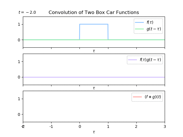
Calculating A Convolution Of Two Box-Car Functions

Setup

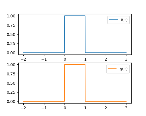
One of the easiest convolution calculations that has a closed-form solution is that of two "box-car" signals.

$f(t)$ is defined by:

$$f(t) = \begin{cases} 1, & \text{for $0 \le t < 1$} \\ 0 & \text{otherwise} \end{cases}$$

And $g(t)$ is exactly the same:

$$g(t) = \begin{cases} 1, & \text{for $0 \le t < 1$} \\ 0 & \text{otherwise} \end{cases}$$

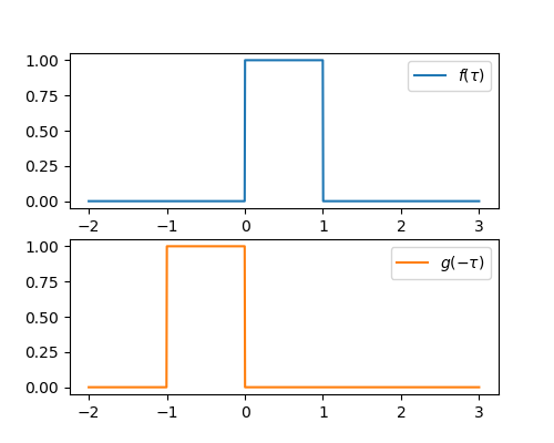
We need to "flip" $g(\tau)$ to give $g(-\tau)$:

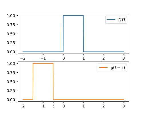
Then we need to shift $g(-\tau)$ by $t$ to give $g(t - \tau)$:

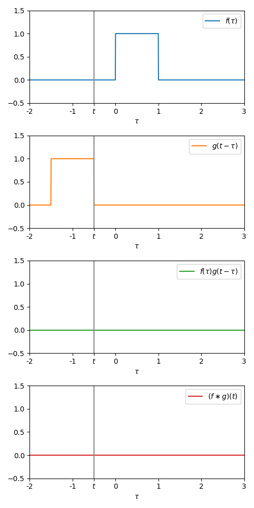
Now we to vary $t$ from $-\infty$ to $+\infty$, and at each $t$, multiply the two signals together $f(\tau)g(t - \tau)$, and calculate the total area under this new signal (mathematically, the integral between $-\infty$ and $+\infty$). This area is the value of the convolution at time $t$.

Obviously, varying $t$ from $-\infty$ to $+\infty$ manually is impossible, but we can break this problem down into sections, and calculate the equation for the convolution function for each section. Because box-car functions are not continuous, we need to break the problem down into sections were each section can describe the convolution in a continuous form.

---

t < 0

When $t < 0$ the two box-cars do not intersect at all, thus the product of $f$ and $g$ is always 0, and thus the area is also 0, which means the value of the convolution function when $t < 0$ is also 0:

$$\int_{-\infty}^{-\infty} f(\tau)g(t - \tau)\,d\tau = 0$$

---

0 <= t < 1

When $0 \le t < 1$, the two box-car functions begin to intersect, with the amount if intersection increasing with $t$. Where they intersect, the product of the two functions is also $1$. This product is shown as the green line below.

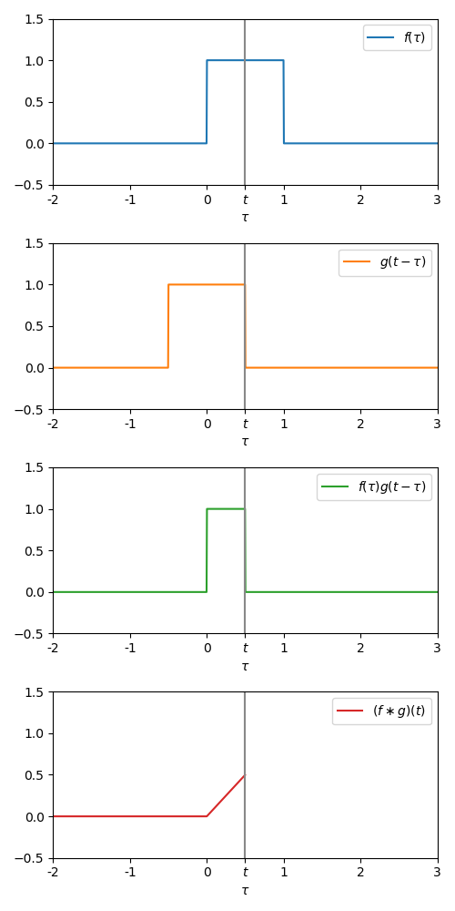
From visual inspection of the green plot, it is obvious that the area under the curve is going to be width*height, which in this case is $(t - 0)*1 = t$. Mathematically this can be calculated by:

$$\begin{align} \int_{-\infty}^{-\infty} f(\tau)g(t - \tau)\,d\tau &= \int_0^t 1*1\,d\tau \\ &= [\tau]_0^t \\ &= t \end{align}$$

---

1 <= t < 2

When $1 \le t < 2$, the functions still intersect, but they are beginning to separate. The area is again width*height, where the width is from $t-1$ to $1$, and the height is still $1$.

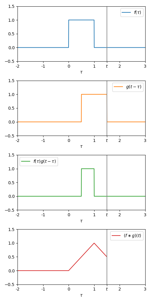
We can calculate a function for the convolution in this interval with:

$$\begin{align} \int_{-\infty}^{-\infty} f(\tau)g(t - \tau)\,d\tau &= \int_{t-1}^1 1*1\,d\tau \\ &= [\tau]_{t-1}^1 \\ &= 1 - (t - 1) \\ &= 2 - t \end{align}$$

---

t >= 2

When $t \ge 2$, the two box-cars do not intersect at all (just like when $t < 0$):

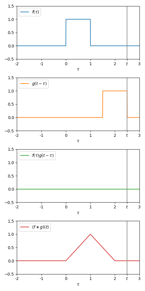
Mathematically we can write this as:

$$\int_{-\infty}^{-\infty} f(\tau)g(t - \tau)\,d\tau = 0$$

---

Combining The Sections

Now that we have derived functions for all of the relevant sections of the convolution function, we can combine them piece-wise to get the final answer:

$$(f \ast g)(t) = \begin{cases} 0, &\text{for $t \le 0$} \\ t, &\text{for $0 \le t < 1$} \\ 2-t, &\text{for $1 \le t < 2$} \\ 0 &\text{fot $t > 2$} \end{cases}$$

An animated .gif showing the convolution of two box-car functions. The value of the convolution function at any time t (bottom line in red) is the amount area shown in red in the middle plot, which is the area under the curve of f(t)g(t) (the two waveforms multiplied together).

Convolution With Unit Impulse (Dirac Delta) Function

Convolution of any function $g(t)$ with the unit impulse function (also known as the Dirac delta function) will always result in $g(t)$ (the original function, unmodified).

$(\delta \ast g)(t) = \int_{-\infty}^{\infty} \delta(\tau) g(t - \tau) = g(t)$

In this sense, the unit impulse function can be considered as the identity function when it comes to convolution (just like the identity matrix in matrix multiplication leaves the original matrix unchanged).

The Convolution Theorem

The convolution theorem states that convolution in the time domain is equal to multiplication in the frequency domain. Mathematically:

$\mathcal{F} \{f \ast g\} = \mathcal{F}\{f\} \cdot \mathcal{F}\{g\}$

We can write the above equation as:

$f \ast g = \mathcal{F}^{-1}\{\mathcal{F}\{f\} \cdot \mathcal{F}\{g\}\}$