Flow Sensors

Caution

This page is in notes format, and may not be of the same quality as other pages on this site.

Flow sensors are sensors that measure the flow rate of a fluid or gas. They are used in a wide range of applications, from measuring the flow of water in a pipe to monitoring the flow of air in an engine.

There are many different physical principles that can be used to measure flow rate. Some common types of flow sensors are:

• Hall effect based flow sensors: These sensors use an impeller with a magnet and a hall effect sensor to detect a rotation of the impeller.
• Ultrasonic flow sensors: These use ultrasonic transducers to measure the flow rate, typically by measuring the difference in transit time of ultrasonic pulses sent with and against the flow.
• Thermal mass flow sensors: They combine a heater element and a temperature sensor to measure the amount of energy absorbed by the fluid as it passes over the heater.
• Differential pressure flow sensors: These utilise the Bernoulli principle to measure the pressure drop across an obstruction as the fluid flows through it.
• Electromagnetic flow sensors: These apply Faraday’s law of induction — a magnetic field is set up across the tube, and a conductive fluid moving through it induces a voltage across a pair of electrodes in the tube wall. The fluid has to be electrically conductive, which means it works well for water but rules out gases and oils.¹

Hall Effect Flow Sensors

MCU Drivers

A microcontroller driver for a hall effect flow sensor is very easy to write, given the simple digital pulse output from the sensor.

Below is some C pseudo code for a hall effect flow sensor driver:

// Access to this has to be atomic. See the notes below.
volatile uint32_t pulseCount = 0;

uint64_t lastMeasurementTime_us = 0;

int main() {
    // Setup the interrupt handler for the hall effect sensor
    configure_interrupt(SENSOR_GPIO_PIN, RISING_EDGE, sensor_isr);

    while(1) {
        uint64_t currentTime_us = get_time_us();

        uint64_t timeSinceLastMeasurement_us = currentTime_us - lastMeasurementTime_us;

        // Assuming there is an atomic_clear() function which
        // clears the atomic variable and returns the previous value
        uint32_t pulseCountCopy = atomic_clear(&pulseCount);

        // F = 6.6 * Q where F is the frequency of the hall effect signal, Q is the flow rate in L/min
        // Q = F / 6.6
        // Q = 1 / (6.6 * t) where t is the period, t = 1 / F
        // Since we have measured N pulses in t_total, t_period = t_total / N,
        // Thus Q = 1 / (6.6 * (t_total / N))
        // Q = N / (6.6 * t_total)
        double flowRate_Lpmin = (double)pulseCountCopy / (6.6 * (double)timeSinceLastMeasurement_us / 1000000.0);
        printf("Flow rate: %.02f L/min\n", flowRate_Lpmin);

        lastMeasurementTime_us = currentTime_us;
        sleep_ms(1000);
    }
}

/**
 * This gets called on the rising edge of the hall effect signal
 */
void sensor_isr() {
    atomic_inc(&pulseCount);
}

If you do not have any atomic variables available, you have two other options:

1. Disable interrupts when reading/clearing the pulse count from main().
2. Use a mutex and lock it when reading/clearing the pulse count from main() (this assumes you are using an RTOS).

Be aware that myVar++ is generally not atomic, even if reading and writing are atomic since ++ (incrementing) involves a read and a write.

Tip

Why does the above code calculate the time since the last measurement and use that in the equation, even though we are sleeping for 1 second between measurements? This is because thread sleep functions are not terribly accurate. Most guarantee that the thread has slept for at least the requested time, but could be longer due to higher priority threads or ISRs running (or even just a bit of latency due to context switching).

I used doubles since I was running on a rather fast microcontroller with FPU support. If using doubles gives you performance issues, you could either use floats or fixed point arithmetic.

I also configured the ISR to be called only on the rising edge of the hall effect signal. This was because triggering on both edges doesn’t really give you any more information, and I didn’t want to make the assumption that the hall effect signal outputted a 50% duty cycle square wave at all speeds (if it strayed far from 50% and you were using data from both edges, you could get some poor flow rate measurements at slower speeds).

High Precision Calibration

Some flow sensors give you more than a basic linear $F = aQ$ equation to convert from pulses to flow rate, to achieve higher accuracy.

One more advanced technique is to provide a calibration curve which tells you what the pulses per litre ($K$) is at different flow rates ($Q$).

For example:

$$K(Q) = a_3 Q^3 + a_2 Q^2 + a_1 Q + a_0$$

where:

• $K(Q)$ is the number of pulses per litre at a flow rate of $Q$ (in L/min)
• $a_0$, $a_1$, $a_2$ and $a_3$ are the coefficients of the polynomial fit to the calibration curve
• $Q$ is the flow rate in L/min

The coefficients $a_0$, $a_1$, $a_2$, and $a_3$ are provided by the manufacturer. To then work out what the flow rate is, you have to perform an iterative calculation, as you need to know $Q$ to work out $K$, but you need $K$ to work out $Q$.

First, you would measure the number of pulses $N$ over a fixed time period $t_{total}$. If $K$ were a constant, the flow rate would just be:

$$Q = \frac{N}{K \, t_{total}}$$

But $K$ depends on $Q$, so the equation to solve is:

$$Q = \frac{N}{K(Q) \, t_{total}}$$

which has $Q$ on both sides. Rather than solving this analytically, it is easier to solve it by fixed-point iteration.

Step 1 — Initial estimate. Use the constant term $a_0$ on its own as a first guess at the pulses per litre. This requires no prior knowledge of $Q$:

$$Q_0 = \frac{N}{a_0 \, t_{total}}$$

Step 2 — Iterate. Re-evaluate the calibration curve at the current flow estimate, and use the resulting $K$ to refine it:

$$Q_{n+1} = \frac{N}{K(Q_n) \, t_{total}}$$

Step 3 — Stop. Repeat until the estimate settles, i.e. when $|Q_{n+1} - Q_n| < \epsilon$ for some tolerance $\epsilon$ (or simply run a fixed number of iterations). Convergence is fast — typically two or three passes — because $K$ varies only mildly across the sensor’s flow range, so each iteration lands close to the last.

Clamping the Calibration Curve

The polynomial is only fitted over the sensor’s valid flow range $[Q_{min}, Q_{max}]$. Outside that range a cubic can extrapolate wildly, so the input to $K$ must be clamped to the fitted range:

$$K(Q) = a_3 \tilde{Q}^3 + a_2 \tilde{Q}^2 + a_1 \tilde{Q} + a_0, \qquad \tilde{Q} = \min\big(\max(Q, Q_{min}), Q_{max}\big)$$

Note that it is only the input to the calibration curve that is clamped, not the reported flow rate. The reported flow rate is still calculated from the true, unclamped pulse count:

$$Q_{n+1} = \frac{N}{K(\tilde{Q}_n) \, t_{total}}$$

So if the measurement implies a flow rate above $Q_{max}$, the pulses per litre is frozen at its boundary value $K(Q_{max})$, but the reported flow rate can still come out above $Q_{max}$. The clamp protects the shape of the correction curve from extrapolating; it is not a limit on the reading itself.

This does mean accuracy degrades outside the valid range, since the correction is no longer tracking the flow rate — below $Q_{min}$ in particular, where the turbine is losing pulses to bearing drag and blade slip, the frozen $K$ under-corrects and the reported flow rate reads low.

Example

You have a flow sensor, and the manufacturer has provided the following calibration curve:

$$K(Q) = a_3 Q^3 + a_2 Q^2 + a_1 Q + a_0$$

where $a_0 = 630.9$, $a_1 = 75.3$, $a_2 = -8.8$ and $a_3 = 0.4$. The manufacturer says the $K(Q)$ calibration equation is valid between 1 and 10 L/min.

In firmware, we have recorded $N = 700$ pulses in 10 seconds. Calculate the volume and flow rate through this sensor.

First, convert the sample window into minutes, to match the units of the calibration curve:

$$t_{total} = \frac{10}{60} = 0.16667\unit{min}$$

We cannot evaluate $K$ yet, because we do not know $Q$. So take the initial estimate using $a_0$ alone:

$$Q_0 = \frac{N}{a_0 \, t_{total}} = \frac{700}{630.9 \cdot 0.16667} = 6.657\unit{L/min}$$

Now iterate, evaluating $K$ at the current estimate and using it to refine the flow rate:

$n$	$K(Q_n)$ (pulses/L)	$Q_{n+1}$ (L/min)	$\lvert Q_{n+1} - Q_n \rvert$
0	860.20	4.883	1.775
1	835.33	5.028	0.145
2	837.88	5.013	0.015
3	837.62	5.014	0.002

Taking a tolerance of $\epsilon = 0.01$ L/min, the estimate has settled by $n = 3$, giving a converged pulses per litre of $K = 837.6$ and a flow rate of:

$$Q = 5.01\unit{L/min}$$

The volume that passed through the sensor during the sample window is then just the pulse count divided by the converged pulses per litre:

$$V = \frac{N}{K} = \frac{700}{837.6} = 0.836\unit{L}$$

As a sanity check, $0.836\unit{L} \div 0.16667\unit{min} = 5.01\unit{L/min}$, which agrees with the flow rate above.

Note how far off the initial estimate was — 6.657 L/min against a true 5.014 L/min, an error of 33%. This is because $a_0$ is the value of the polynomial at $Q = 0$, which is well below the flow rate we actually ended up at. The iteration is doing real work here; a single pass would not have been enough.

Note that every estimate — including the initial 6.657 L/min — landed inside the manufacturer’s valid range of 1 to 10 L/min, so the clamp described above never engaged. Had the initial estimate come out above 10 L/min, $K$ would have been evaluated at $Q_{max} = 10$ L/min for that first pass instead.

Example Hall Effect Flow Sensors

YF-Bx

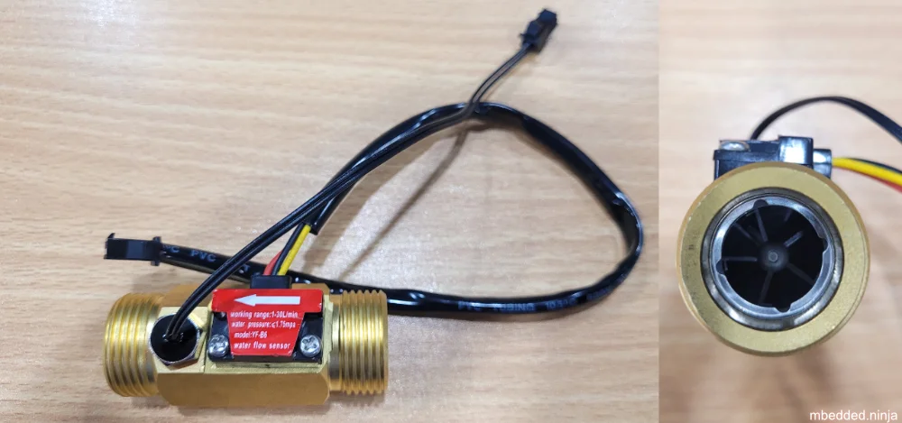
YF-Bx is a family of hall effect based flow sensors mounted in a small piece of brass tubing (DN15 or DN20, i.e. ½” or ¾”). Depending on the variant, they measure flow rates between 1 and 25 or 1 and 30 L/min. The YF-Bx family have a working voltage of 5V to 15V(DC) and the G1&x family have a working voltage of 5V to 24V(DC).

There are three wires:

• Red: +VCC
• Black: GND
• Yellow: Signal

The yellow signal wire outputs a digital signal which transitions between high and low a fixed number of times per revolution of the impeller (using the hall effect sensor). It has a duty cycle of 50% ±10%.

A waveform from an oscilloscope showing the output of a YF-B6 flow sensor when blowing through it. The air speed was slowing down from left to right.

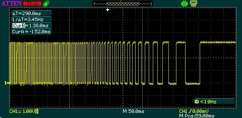
Note how the duty cycle drifts well away from 50% towards the slow (right-hand) end of the capture — the high time becomes noticeably longer than the low time. This is why the driver above triggers on one edge only.

The rate is typically expressed as a frequency. For example, the YF-B6 datasheet describes a frequency of F=6.6*Q(Q=L/MIN).² F is the measured frequency of the hall effect signal, and Q is the flow rate in L/min. In a microcontroller, you would typically set up a GPIO interrupt on the sensor pin, and accumulate the number of pulses over a fixed period of time (e.g. check once per second). To calculate the flow rate, we would need to re-arrange the equation. Let’s also substitute $F$ for the period $t$ ($t = \frac{1}{F}$) since that’s what we’ll actually measure.

$$\begin{align*} F &= 6.6 \cdot Q \\ Q &= \frac{F}{6.6} \\ &= \frac{1}{6.6t_{period}} \\ \end{align*}$$

where:

• $F$ is the frequency of the hall effect signal in Hz
• $Q$ is the flow rate in L/min
• $t_{period}$ is the time between pulses in seconds

As you normally want to accumulate a number of pulses over a fixed period of time (e.g. 1s), and then calculate the flow rate, you need to modify the equation slightly. Let’s call the number of pulses $N$ and the total time period these were measured over $t_{total}$.

$$t_{period} = \frac{t_{total}}{N}$$

where:

• $N$ is the number of pulses measured over a fixed period of time
• $t_{total}$ is the total time period over which the pulses are measured

So therefore:

$$\begin{align*} Q &= \frac{1}{6.6 \cdot \frac{t_{total}}{N}} \\ &= \frac{N}{6.6 \cdot t_{total}} \\ \end{align*}$$

Caution

Some websites write the equation as F=(6.6*Q)Q=L/MIN±3%. This is terribly confusing! The bad placement of the brackets and lack of spaces makes it look like the equation is a quadratic (i.e. F=6.6Q^2).

The other difference between the two families is the tube material: the YF-Bx parts have a brass tube, whilst the G1&x parts have a plastic one.

Photo of the outside and inside of the YF-B6 flow sensor.

The table below shows the core specifications for the flow sensors in the YF-Bx and G1&x families. For the frequency equation, $F$ is the frequency of the hall effect signal in Hz, $Q$ is the flow rate in L/min.

Specifications for the YF-Bx and G1&x family of flow sensors.³

Type	Dimensions (DN)	Working Voltage	Flow Rate Range	Frequency Eq.	Length	Male & Female	Length of Thread	Material
YF-B1	DN15	5V to 15V(DC)	1 to 25L/min	-	44mm	Double Male	10mm	Copper
YF-B2	DN15	5V to 15V(DC)	1 to 25L/min	-	50mm	Male in Female out	10mm	Copper
YF-B3	DN15	5V to 15V(DC)	1 to 25L/min	-	66mm	Double Male	18mm	Copper
YF-B4	DN15	5V to 15V(DC)	1 to 25L/min	-	66mm	Male in Female out	10mm	Copper
YF-B5	DN20	5V to 15V(DC)	1 to 30L/min	F=6.6*Q	50mm	Double Male	10mm	Copper
YF-B6	DN20	5V to 15V(DC)	1 to 30L/min	F=6.6*Q	60mm	Double Male	11mm	Copper
YF-B7	DN15	5V to 15V(DC)	1 to 25L/min	-	66mm	Double Male	10mm	Copper
G1&2	DN15	5V to 24V(DC)	1 to 30L/min	-	-	Double Male	-	Plastic
G3&4	DN20	5V to 24V(DC)	1 to 60L/min	-	-	Double Male	-	Plastic
G1&8	-	5V to 24V(DC)	0.3 to 6L/min	-	-	-	-	Plastic
M11*1.25	-	5V to 24V(DC)	0.3 to 6L/min	-	-	-	-	Plastic

There is also the YF-S201 flow sensor which seems related.

I have found some significant accuracy issues when using this type of sensor, specifically with the YF-B5. The quoted accuracy as per its datasheet is $\pm 3\%$ over a flow rate range of 1 to 30L/min.⁴ However, I have found the error to be closer to 1L/min when reading a low flow rate of 1L/min, with the accuracy improving as the flow rate increases. The calibration curve below is fitted against measurement data from 3 YF-B5 flow sensors. The dotted black line shows where we would expect the points to be if the sensor followed the datasheet’s quoted equation and accuracy. The dots are measurements from the 3 sensors vs. the actual flow rate (as measured by an expensive and accurate flow meter). The red line is the linear least squares best fit line through the data.

A calibration curve fitted against measurement data from 3 YF-B5 flow sensors.

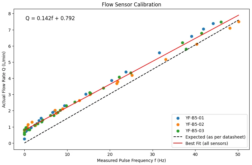
As shown in the calibration curve above, the equation for the best fit line is:

$$\begin{align*} Q = 0.142f + 0.792 \end{align*}$$

where:

• $Q$ is the flow rate (in L/min)
• $f$ is the frequency (in Hz) of the flow sensor output

Using this linear best fit equation in firmware to convert from the pulses per second to a flow rate should give a much more accurate flow rate than the $F = 6.6Q$ ($Q = 0.152f$) equation provided in the datasheet.

Tiny Flow Sensors

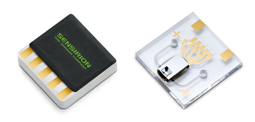
Tiny flow sensors exist in chip-size packages. These are in a group of products called MEMS (micro-electro-mechanical system) devices.

Sensirion makes small 10 × 10mm liquid flow sensors (the LPP10 and LPG10). They are based on thermal MEMS elements. They can measure between 0 and 1000uL/min (1mL/min), with a resolution that can be as low as 0.5nL/min. It has a response time of 40ms/sample. It is compatible with H2O, methanol, ethanol, and blood.

A small 10 × 10mm thermal MEMS-based flow sensor (LPG10, LPP10) from Sensirion. Image from http://www.sensirion.com/en/products/liquid-flow-sensors/customized-solutions/.

Electromagnetic Flow Sensors

Electromagnetic flow sensors (aka magnetic-inductive (MID), magneto-inductive, mag meter) measure liquid speed by using Faraday’s Law of electromagnetic induction. The law states that when a conductor moves through a magnetic field, a voltage is induced in the conductor. In an electromagnetic flow sensor, the moving liquid is the conductor, and the sensor generates a magnetic field around it.¹

The main advantages of electromagnetic flow sensors are that they are unaffected by changes in pressure, temperature or viscosity, and have no moving parts. This also means little to no pressure drop across the meter, and they cope well with dirty or corrosive media.⁵

The catch is the conductivity requirement. The liquid typically has to exceed something like 5 to 20 µS/cm (Siemens being a measure of conductivity), which is fine for acids, caustics and salt solutions, but rules out deionised water, oils and alcohols.⁵ A few other things to be aware of when installing one:

• The pipe must be running full — a partially filled pipe reads low.
• Allow straight pipe runs either side of the meter, on the order of 5 pipe diameters upstream and 2 to 3 downstream.
• The induced signal is only millivolts, so it is easily swamped by noise, and nearby magnetic fields will interfere with it.

Accuracy is typically around 0.5%, with a turndown ratio (the ratio of the highest to lowest flow rate it can measure) of roughly 40:1. This is noticeably worse than the 250:1 an ultrasonic meter can manage.⁵

Further Reading

See Hall effect sensors for more information on the hall effect principle and how Hall effect sensors are built.

See Encoders for more information on how encoders work and how they can be connected to a microcontroller.

Footnotes

1. Endress+Hauser (2024, Dec 3). Understanding electromagnetic flowmeters: Features and benefits. Retrieved 2026-08-04, from https://www.endress.com/en/support-overview/learning-center/flow-measuring-principle-emf. ↩ ↩²

2. Seeed Studio. Water Flow Sensor YF-B6 [datasheet]. Retrieved 2025-02-25, from https://media.digikey.com/pdf/data%20sheets/seeed%20technology/114991176_web.pdf. ↩

3. Seeed Studio. Home / The Devices / Data Collection Systems / Energy Management Units / Water Flow Sensor YF-B6 [product page]. Retrieved 2025-02-24, from https://www.seeedstudio.com/Water-Flow-Sensor-YF-B6-p-2883.html. ↩

4. Seeed Studio. Water Flow Sensor YF-B5 [datasheet]. Retrieved 2025-04-08, from https://mm.digikey.com/Volume0/opasdata/d220001/medias/docus/5670/1597_Seeed%20114991175.pdf. ↩

5. Heather Collins. Understanding Magnetic Flow Meters & How They Work. KOBOLD Instruments. Retrieved 2026-08-05, from https://koboldusa.com/articles/type-of-flow-meters/understanding-magnetic-flow-meters/. ↩ ↩² ↩³