Basic Signal Types

Overview

This page serves to be a tutorial on the basic types of signals/waveforms you will come across in engineering.

All usages of trigonometric functions such as \(\sin()\) and \(\cos()\) below assume angles measured in radians, not degrees.

This page assumes basic understanding of trigonometry and complex numbers.

Real Sinusoidal Signals

A real sinusoidal signal has the general form:

$$ f(t) = A \sin ( \omega t + \theta ) $$

where:
\(A\), \(\omega\), and \(\theta\) are real numbers

An example sinusoidal where \( f(t) = 2\sin(2t + \frac{\pi}{4}) \) is shown below:

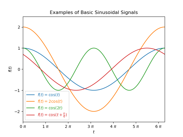
\(A\) controls the amplitude of the signal. A negative number will invert the signal. A value of \(A = 1\) will give an amplitude of \(1\).

\(\omega\) controls the period/frequency of the signal. A value of \(\omega = 1\) gives a period of \(2\pi\). Doubling \(\omega\) doubles the frequency.

\(\theta\) controls the offset of the signal along the x-axis. A positive value shift the signal to the left, a negative value shifts the signal to the right.

Sinusoidal signals normally arise in systems that conserve energy, such as an ideal mass-spring system (no damper or frictional forces!), or an ideal LC circuit (no resistive losses).

Complex sinusoidal signals are introduced after exponential signals are explained.

Exponential Signals

The general form for an exponential signal is:

$$ f(t) = Ae^{\lambda t} $$

where:
\(A\), \(\lambda\) are complex numbers

Real Exponential Signals

Below are some examples of real exponential signals, showing how varying \(A\) and \(\lambda\) (limited to real numbers only) effect the waveform shape.

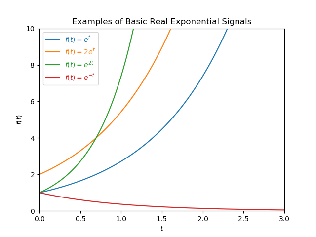
When \(\lambda > 1\), the signal exhibits exponential growth (this typically represents an unstable signal). When \(\lambda < 1\), the signal exhibits exponential decay (this typically represents a stable signal).

Complex Exponential Signals

If the restriction that \(A\) and \(\lambda\) must be real numbers is removed from the general form for an exponential signal, and they are now complex numbers, a different class of signals arise. We substitute \(\lambda\) in the general form for a exponential signal for the complex number \(z = \sigma + i\omega \) to give:

$$ f(t) = Ae^{(\sigma + i\omega)t} $$

where:
\(\sigma\) is the attenuation constant
\(\omega\) is the angular frequency

Recap Euler’s formula:

$$ e^{it} = \cos(t) + i\sin(t) $$

Also,

$$ A = |A|e^{i\theta} $$

This allows us to separate out the real and imaginary parts into individual terms:

$$\begin{align} f(t) &= Ae^{\lambda t} \\ &= |A|e^{i\theta}e^{(\sigma + i \omega)t} \\ &= |A|e^{i\theta}e^{\sigma t + i \omega t} \\ &= |A|e^{i\theta}e^{\sigma t}e^{i \omega t} \\ &= |A|e^{\sigma t}e^{i (\omega t + \theta)} \\ &= |A|e^{\sigma t} \cos(\omega t + \theta) + i |A|e^{\sigma t} \sin(\omega t + \theta) \end{align}$$

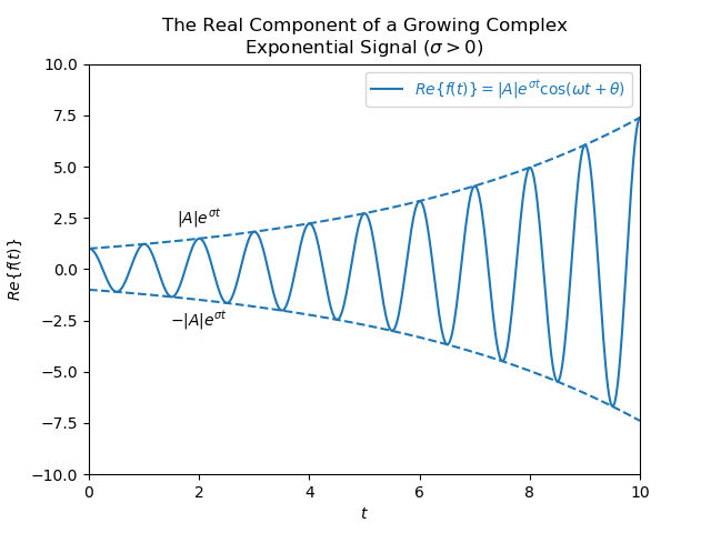
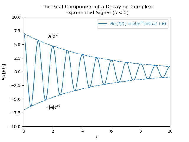
Below are graphs of the real component of both growing and decaying complex exponential signals. You can see how the signal is enveloped by \(\pm |A|e^{\sigma t}\). This is because the signal is the product of an exponential component and a \(\cos()\) component, and the \(\cos()\) component always varies between \(-1\) and \(1\).

Heaviside (Unit-Step) Function

The Heaviside function, named after Oliver Heaviside (also known as the unit-step function) can be defined as:

$$ f(t) = \begin{cases} 0, & \text{for $t < 0$} \\ 1 & \text{for $t > 0$} \end{cases} $$

The Heaviside function looks something like the signal below, however the point at \(H(0)\) can be drawn in different ways (more on that below):

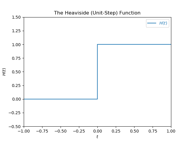
Oliver Heaviside used his equation to calculate the current in an electrical circuit when it is first switched on ^hello.

The Different Conventions For H(0)

The value of Heaviside function at 0 (\(H(t)\) at \(t = 0\)) depends on the implementation or use of the function. The different values are described below. However, it is worth noting that the value of \(H(0)\) is of no importance for most use cases of the Heaviside function, as it is commonly used as a windowing function in integration (or distribution).

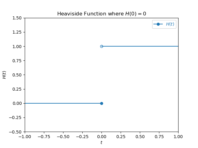
H(0) = 0

$$ H(t) = \begin{cases} 0, & \text{for $t <= 0$} \\ 1 & \text{for $t > 0$} \end{cases} $$

This is how the NIST DLMF (Digital Library of Mathematical Functions) defines the Heaviside function (see section 1.16.13). This version of the Heaviside function is left-continuous at \(t = 0\) but not right continuous.

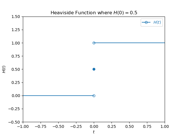
H(0) = 0.5

If the convention \(H(0) = 0.5\) is used, the Heaviside function defined as:

$$ H(t) = \begin{cases} 0, & \text{for $t < 0$} \\ \frac{1}{2}, & \text{for $t = 0$} \\ 1 & \text{for $t > 0$} \end{cases} $$

This is the version of the Heaviside function which seems to be most often used. The Numpy documentation for numpy.heaviside() states that \(H(0) = 0.5\) is often used. This format of the Heaviside is also closely related to the signum function (the function used to extract the sign of a real number), by the following equation (shifted up by 1 and then halved in magnitude):

$$ H(t) = \frac{1 + sgn (t)}{2} $$

Drawn on a graph it looks like:

H(0) = 1

$$ H(t) = \begin{cases} 0, & \text{for $t < 0$} \\ 1 & \text{for $t >= 0$} \end{cases} $$

\(H(0) = 1\) is how ISO 80000-2:2009 defines the Heaviside function ^hello. This version of the Heaviside function is right-continuous at \(t = 0\) but not left continuous. It also allows the Heaviside function to be defined as the integration of the unit impulse (Dirac delta) function:

$$ H(t) = \int_{-\infty}^{t} \delta(x) dx $$

Drawn on a graph it looks like:

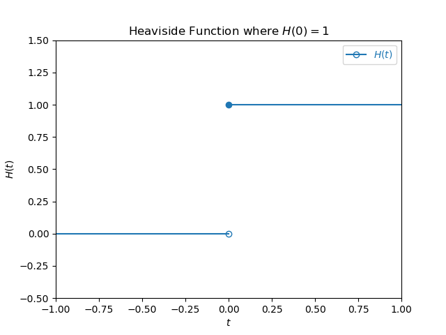
The Heaviside function is usually defined like this when used in the context of cumulative distributions for statistical purposes.

H(0) = [0, 1]

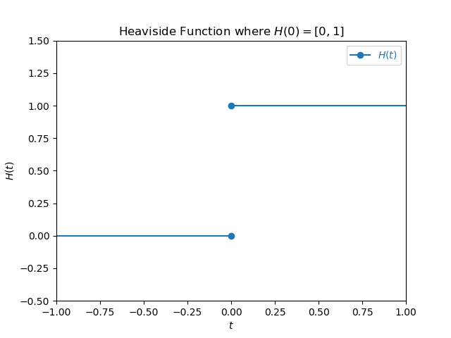
\(H(0) = [0, 1]\) is when the Heaviside equals both \(0\) and \(1\) (a set) at \(t = 0\). This approach is not as common, but is used in optimization and game theory^hello.

Drawn on a graph it looks like:

Shifted Heaviside

TODO

Unit Impulse (Dirac Delta) Function

The unit-impulse function (known as a the Dirac delta function in the mathematical world) is defined as:

$$ f(t) = 0 \text{ for } t \neq 0 \text{ and} \\ \int_{- \infty}^{\infty} f(t) dt = 1 $$

The unit-impulse function is \(0\) everywhere except for \(t = 0\) where it is infinite.

References

• https://www.quora.com/What-is-the-value-of-the-unit-step-function-at-T-0
• https://www.iso.org/standard/31887.html
• https://en.wikipedia.org/wiki/Oliver_Heaviside