Understanding Logistic Regression

Article by:

Date Published:	February 21, 2020
Last Modified:	March 21, 2020

Overview

Logistic regression (or logit regression) is a very common and popular algorithm that is used in machine learning. It is used for making binary categorical predictions, such as “is it going to rain today?” or more precisely, it can be used to give a percentage chance of it raining today. Logistic regression can also be extended to make many-option categorical predictions, such as “is it more likely to be sunny, overcast, or rainy today?”.

Probability and Odds

Before learning about logistic regression, it is wise to understand the terms probability and odds.

We’ll start with a real simple equation. The probability $P$ of a binary event occurring is:

$$ P $$

The probability of a binary event not occurring must then be:

$$ 1 - P $$

The Odds is defined as the ratio of success to the ratio of failure.

$$ O = \frac{P}{1 - P} $$

It should be clear from the above equation that if $P$ can vary in the range $[0, 1]$ then $O$ can vary in the range $[0, \infty]$. The higher the odds, the higher the chance of success. This should sound very familiar to gamblers, who use this term frequently.

Why Use The Logarithmic Function?

The reason we introduce the $ln()$ function into the equation begins to make sense once you understand basic linear regression, which can be used to predict the probability of continuous target variables. The basic equation defining linear regression involving just one predictor $x$ and the outcome $y$ is:

$$ y = \beta_0 + \beta_1 x\\ -\infty < x < \infty\\ -\infty < y < \infty $$

where:
$\beta_n$ are the coefficients
$x$ is the predictor
$y$ is the outcome

The problem with using linear regression for making binary categorical predictions (i.e. true/false) is that $y$ can vary from $-\infty$ to $+\infty$. We really want $y$ to range from $0$ to $1$. When varying between $0$ and $1$, this tells us the probability of the target being true or false. For example, if $y=0.7$ this would say there is a 70% chance of the target being true, and conversely a 30% chance of the target being false.

To make things less confusing, we will replace $y$ which is used to represent a continuous target variable with $P$ (for probability), which is used to represent the probability:

$$ P = \beta_0 + \beta_1 x\\ -\infty < x < \infty\\ 0 \leq P \leq 1 $$

Notice a problem? This limits of the LHS and RHS of the equation don’t match up! This is where we begin to understand why the log function is introduced. We will try and modify the RHS such that it has the same range as the LHS ($-\infty$ to $+\infty$). What if we replace the probability $P$ on the LHS with the odds $O$:

$$ O = \beta_0 + \beta_1 x\\ -\infty \leq x < \infty\\ 0 \leq O < \infty $$

where:
$O$ are the odds

We are getting closer! Now the RHS varies from $0$ to $\infty$ rather than from just $0$ to $1$. So how do we modify a number which ranges from $0$ to $1$ to range from $-\infty$ to $+\infty$? One way is to use the ln() function! (to recap some mathematics, the ln of values between 0 and 1 map from $-\infty$ and $0$, and the ln of values from $1$ to $\infty$ map to $0$ to $\infty$.)

$$ \ln(O) = \beta_0 + \beta_1 x\\ -\infty < x < \infty\\ -\infty < \ln(O) < \infty $$

The ranges on both sides of the equation now match! The base of the logarithm does not actually matter. We choose to use the natural logarithm ($\ln$) but you could use any other base such as base 10 (typically written as $log_{10}$ or just $log$).

Now we can see why it’s called logistic regression, and why it is useful.

However, the equation is usually re-arranged with $P$ on the LHS.

$$\begin{align} \ln(O) &= \beta_0 + \beta_1 x\\ O &= e^{\beta_0 + \beta_1 x} &\text{Take the exponential of both sides}\\ \frac{P}{1 - P} &= e^{\beta_0 + \beta_1 x} &\text{Substitute $O$ as per equation XXX}\\ P &= e^{\beta_0 + \beta_1 x}(1 - P) &\text{Multiply both sides by $(1 - P)$}\\ P &= e^{\beta_0 + \beta_1 x} - Pe^{\beta_0 + \beta_1 x} &\text{Expand RHS}\\ P + Pe^{\beta_0 + \beta_1 x} &= e^{\beta_0 + \beta_1 x} &\text{Move all terms with $P$ to the LHS}\\ P(1 + e^{\beta_0 + \beta_1 x}) &= e^{\beta_0 + \beta_1 x} &\text{Factor the $P$}\\ P &= \frac{e^{\beta_0 + \beta_1 x}}{1 + e^{\beta_0 + \beta_1 x}} &\text{Divide both sides of equation by $1 + e^{\beta_0 + \beta_1 x}$}\\ P &= \frac{1}{\frac{1}{e^{\beta_0 + \beta_1 x}} + 1} &\text{Divide top and bottom of RHS fraction by $e^{\beta_0 + \beta_1 x}$}\\ P &= \frac{1}{1 + e^{-(\beta_0 + \beta_1 x)}} &\text{Use rule $\frac{1}{e^x} = e^{-x}$} \end{align}$$

As you can see from above, $P$ is now a form of a sigmoid function.

What Does The Logistic Function Look Like?

So we have the basic logistic function equation:

$$ P = \frac{1}{1 + e^{-(\beta_0 + \beta_1 x)}} $$

where:
$\beta_0$ and $\beta_1$ are constants

What happens as we change $\beta_1$?

It changes the shape of the curve, starting-off looking like a linear line, and progressively getting closer to looking like a step function. This $\beta_1$ term is analogous to the slope $m$ in linear regression.

What happens as we change $\beta_0$?

This is analogous to the y-intercept $c$ in linear regression, except that $\beta_0$ shifts the curve along the x-axis.

Worked Example

We can use logistic regression to perform basic “machine learning” tasks. We will use the famous Iris dataset, and write the code in Python, leveraging sklearn’s logistic regression training class and various reporting tools. The Iris dataset is popular enough that it’s bundled with a number of Python libraries, including seaborn (which is where we will grab it from):

1
2
3
4
import seaborn as sns
from sklearn.linear_model import LogisticRegression
from sklearn.metrics import accuracy_score, classification_report
from sklearn.model_selection import train_test_split

1
2
3
4
data = sns.load_dataset('iris')
print(data.shape[0])
# 150
data.head())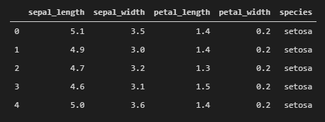

Split the data into the features x and the target y:

1
2
x = data.iloc[:, 0:-1] # All columns except "species"
y = data.iloc[:, -1] # The "species" column

Now split the data into training and test data:

1
x_train, x_test, y_train, y_test = train_test_split(x, y, test_size=0.2, random_state=0)

Let’s train the model:

1
2
model = LogisticRegression()
model.fit(x_train, y_train) # Training the model

Make predictions:

1
2
predictions = model.predict(x_test)
print(predictions)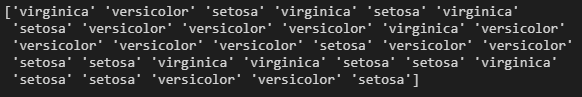

The predictions of the type of Iris for the test data.

Print a “classification report”:

1
print(classification_report(y_test, predictions))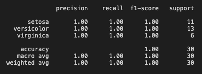

The classification report for our logistic regression model.

For someone new to categorization, these terms in the classification report can be confusing. This is what they mean¹:

The precision is how well the classifier is at labelling an instance positive when it was actually positive. It can be thought of as: “For all instances labelled positive, what percentage of them are actually correct?
$$ precision = \frac{true\,positive}{true\,positive + false\,positive} $$
The recall is the ability for a classifier to find all true positives. It can be though of as: “For all instances that where actually positive, what percentage were labelled correctly?”
$$ recall = \frac{true\,positive}{true\,positive + false\,negative} $$
The f1-score is the harmonic mean of the precision and recall. Personally I find this the most difficult metric to understand intuitively. It is a score which incorporates both the precision and recall, and varies between 0 and 1.
The support is the number of actual occurrences of a class in a specific dataset.

And let’s print the accuracy score:

1
2
print(accuracy_score(y_test, predictions))
# 0.9666666666666667

pocky

External Resources

https://towardsdatascience.com/logit-of-logistic-regression-understanding-the-fundamentals-f384152a33d1

https://www.scikit-yb.org/en/latest/api/classifier/classification_report.html ↩︎

Authors

Geoffrey Hunter

Dude making stuff.

Twitter

GitHub

This work is licensed under a Creative Commons Attribution 4.0 International License .