Exponential Moving Average (EMA) Filters

The exponential moving average (EMA) filter is a discrete, low-pass, infinite-impulse response (IIR) filter. It places more weight on recent data by discounting old data in an exponential fashion, and behaves similarly to the discrete first-order low-pass RC filter.
Unlike a simple moving average (SMA) filter, most EMA filters are not windowed, and the next value depends on all previous inputs. Thus most EMA filters are a form of infinite impulse response (IIR) filter, whilst a SMA is a finite impulse response (FIR) filter. There are exceptions, and you can indeed build a windowed exponential moving average filter where the coefficients are weighted exponentially.
EMA Equation
The difference equation for an exponential moving average filter is:
where:
is the output ( denotes the sample number)
is the input
is a constant which sets the cutoff frequency (a value between and )
Notice that the calculation does not require the storage of past values of and only the previous value of , which makes this filter memory and computation friendly (especially relevant for microcontrollers). Only one addition, one subtraction, and two multiplication operations are needed. If you are really tight on cycles, you can rearrange the difference equation into the algebraically-equivalent form , which needs just one addition, one subtraction, and a single multiplication.
The constant determines how aggressive the filter is. It can vary between and (inclusive). As , the filter gets more and more aggressive, until at , where the input has no effect on the output (if the filter started like this, then the output would stay at ). As , the filter lets more of the raw input through, resulting in less filtered data, until at , where the filter is not “filtering” at all (pass-through from input to output).
The filter is called exponential because the weighted contribution of previous inputs decreases exponentially the further the input is away in time. This can be seen in the difference equation if we substitute in previous inputs:
The following code implements a basic EMA filter in C++, suitable for microcontrollers and other embedded devices:
#include <stdio.h>#include <cstdint>
class EmaFilter{public:    EmaFilter(double alpha) :        m_alpha(alpha), m_lastOutput(0.0) {}
    double Run(double input)    {        m_lastOutput = m_alpha * input + (1 - m_alpha) * m_lastOutput;        return m_lastOutput;    }private:    double m_alpha;    double m_lastOutput;};
int main() {    EmaFilter emaFilter(0.5);
    for(uint32_t i = 0; i < 20; i++)    {        double input = 1.0;        double output = emaFilter.Run(input);        printf("%f\n", output);    }}
When setting alpha=0.5 and hardcoding all input to 1.0 (which means a step change from 0.0 to 1.0 at t=0), it prints the following:
0.5000000.7500000.8750000.9375000.9687500.9843750.9921880.9960940.9980470.9990230.9995120.9997560.9998780.9999390.9999690.9999850.9999920.9999960.9999980.999999This example can be modified and run at https://replit.com/@gbmhunter/cpp-ema-filter.
Frequency Response
The frequency response of the EMA filter can be found by using the Z transform. If we start with the time-domain equation for an EMA filter:
And then take the Z transform of it:
Then re-arrange to find the transfer function :
This transfer function can be used to create bode plots of the magnitude and phase response of the EMA filter. The below bode plot shows the response of an EMA filter with . The x-axis frequency is the normalized frequency, in units of , which makes the plot applicable for any sampling frequency.
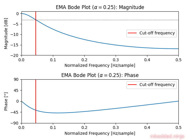
The cut-off frequency (-3dB point) of an EMA filter is given by1:
where:
is the sampling frequency in
An important consequence of this is that the filter’s response is dependent both on and the sampling frequency. Remember that if you adjust the sampling frequency, you also have to adjust to keep the same response.
Note that not all valid values of will result in a valid cut-off frequency. This is when the filter response is so gradual that it does not drop to -3dB or below before the Nyquist frequency. Mathematically, this is when:
and thus the inverse cosine function is undefined. The expression above becomes greater than 1 when is at or above1:
Interactive EMA Filter Explorer
The widget below lets you explore both sides of the EMA filter at once. Drag and watch how it trades smoothing against responsiveness in the Time domain tab, then switch to the Frequency response (Bode) tab to see the same shape the magnitude and phase response. Push above and the -3dB cut-off marker disappears, illustrating the “no valid cut-off before Nyquist” condition derived above.
Impulse Response
The discrete unit sample function is defined as:
If we use this as our input into :
Given the unit sample function is 0 at most points, the only sum term that matters is when , so we can simplify this to:
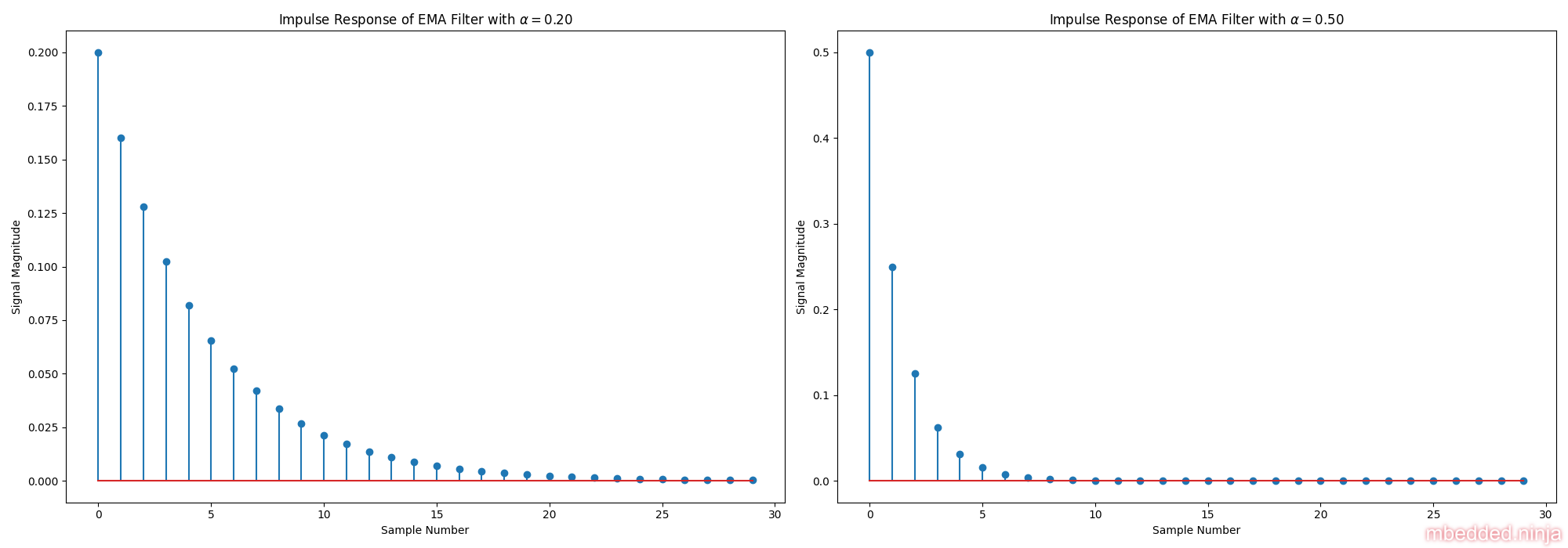
From this, we can plot what the response will look like for impulse as the input. As you can see in the following graph, the output starts off at and then decays towards 0. A larger alpha makes the initial response larger but also the decay faster.
Time Constant
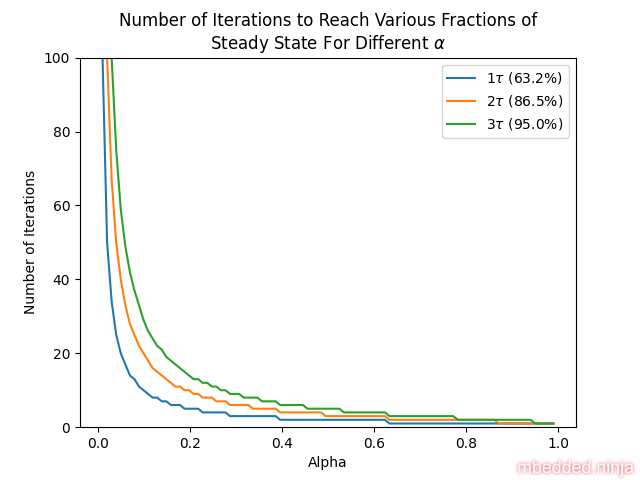
Related to the frequency response and the impulse response, you can define a time constant for the EMA filter. The time constant is the time it takes for the output to reach (63.2%) of the steady state value. This is a placeholder for the reference: fig-ema-time-constant shows the number of iterations required to reach a given fraction of steady state for different values. This is assuming a step change in the input from 0 to 1 at .
Initializing (Priming) The Filter
When initializing the filter, the initial value of is important. If you set it to 0, then the filter will take a while to “warm up” and reach the correct output. If you set it to the first input value, then the filter will get a “head start”. This may or may not be important for your application. I typically have a boolean flag called firstTime which is set to true when the filter is first created, and then set to false after the first input is processed. On the first pass, the filter just sets the output to the input . I call this priming the filter, to avoid confusion with “initialisation” of an object (i.e. constructor).
Here is an example of the C++ class from above but reworked to include priming:
class EmaFilterWithPriming{public:    EmaFilterWithPriming(double alpha) :        m_alpha(alpha), m_lastOutput(0.0), m_firstRun(true) {}
    double Run(double input)    {        if (m_firstRun)        {            m_firstRun = false;            m_lastOutput = input; // Bypass filter and prime with input        }        else        {            m_lastOutput = m_alpha * input + (1 - m_alpha) * m_lastOutput;        }        return m_lastOutput;    }private:    double m_alpha;    double m_lastOutput;    bool m_firstRun;};
This example can be modified and run at https://replit.com/@gbmhunter/cpp-ema-filter.
Further Reading
https://stratifylabs.co/embedded%20design%20tips/2013/10/04/Tips-An-Easy-to-Use-Digital-Filter/ is a great page explaining the exponential moving average filter.
References
Footnotes
-
Andy Walls (2017, Apr 22). Exponential moving average cut-off frequency (Q/A). StackExchange: Signal Processing. Retrieved 2022-05-25, from https://dsp.stackexchange.com/questions/40462/exponential-moving-average-cut-off-frequency. ↩ ↩2