Analogue Filters

Child Pages

Filter Tunings

Sallen-Key Filters

Overview

Passive vs. Active

Even in the pass-band, passive filters almost always increase the impedance of the signal, post filter. For a trace on a circuit board, this actually makes the post-filter trace more susceptible to picking up external noise. For this reason, when using a passive filter to filter out induced noise of a sensitive trace, always place a passive filter as close as possible to the receiving end of the signal (e.g. as close as possible to an ADC pin on a microcontroller).

Low-pass filters have an additional advantage when used on the analogue outputs from microcontrollers. If the DAC does not work properly for some reason (assuming you are using a DAC), you can sometimes implement the desired behaviour by using PWM instead. With the cut-off frequency set correctly, the PWM signal will be filtered so that a DC voltage proportional to the duty cycle remains, which is what you wished to implement with the DAC in the first place.

Active filters are electronic waveform filters which require their own power source (such as any filter powered with an op-amp), as opposed to passive filters (such as RC filters) which do not require an external power source. Active filters allow higher roll-of and better transfer characteristics than passive filters, but require more componentry and consume power.

Filter Topologies vs. Tunings

• Filter types describe the purpose of the filter. Filter types include low-pass, high-pass, band-pass, notch (band reject), and all-pass.
• Filter topologies define the what components go where. Filter topologies include
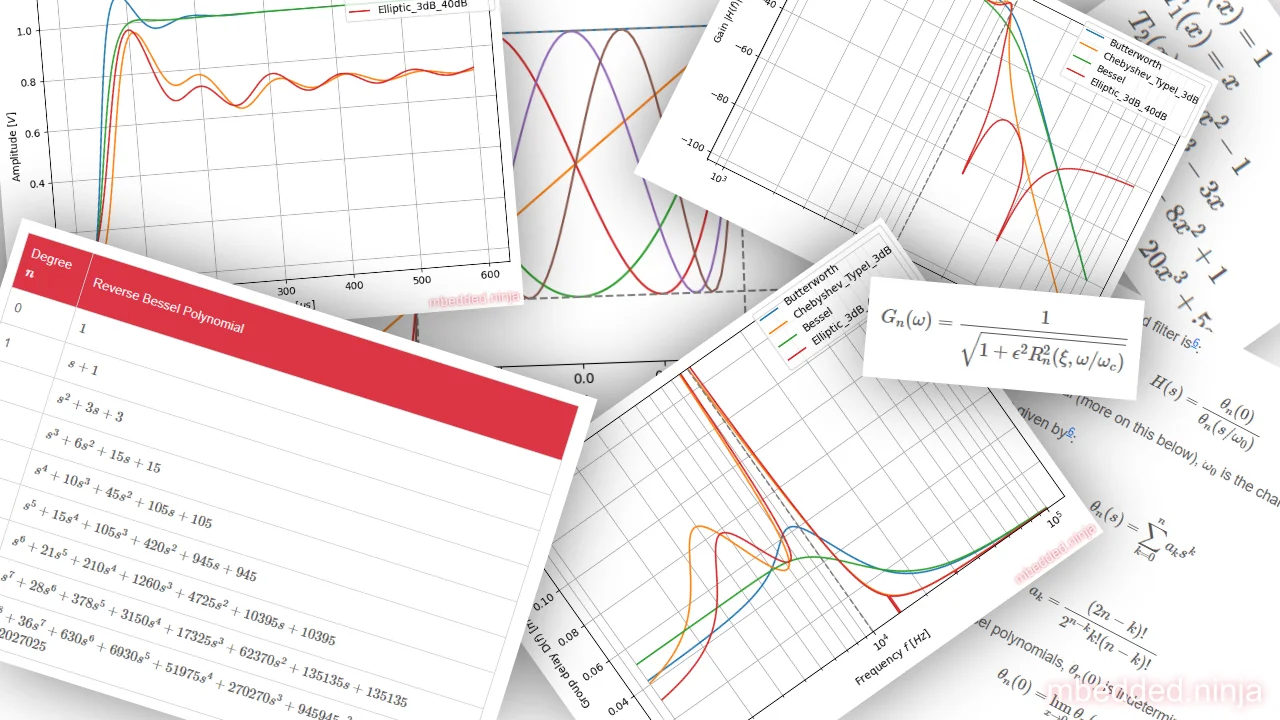
• Filter tunings define the values of the components in a particular topology. Filter tunings include Butterworth, Chebyshev and Bessel.

Filter Parameters

Cutoff Frequency (fc)

The cutoff frequency (a.k.a. corner frequency or break frequency) is the frequency which marks the transition from a pass band to a stop band. It marks the frequency at which the energy (whether it be voltage, current or both) stops being passed through and begins being blocked. For any real filter, there is a transition from the passband to the stopband, as so the cutoff frequency is usually defined at the “-3dB” point — the point at which the signal degrades to -3dB (half power) of the nominal passband value.

The symbol \(f_c\) is usually used to represent the cutoff frequency. Sometimes you may see \(f_{-3dB}\) instead.

Gain Factor (K)

At frequencies \(f << f_c\), the circuit multiplies the input signal by gain factor K.

Component Spread

Component spread is a measure of ratio between the highest and lowest valued components required to construct a filter. Low component spread is a good property for a filter to have, as it aids manufacturability.

Filter Optimizations

Filter optimizations maximize a certain characteristic of a filter topology, such as maximum pass-band flatness or steepest roll-off. Butterworth, Chebyshev and Bessel are examples of filter optimizations.

1st Order Filters

First-Order Low-Pass RC Filter

Schematic

The below schematic shows a first-order low-pass RC filter consisting of a single series resistor and then a single capacitor to ground.

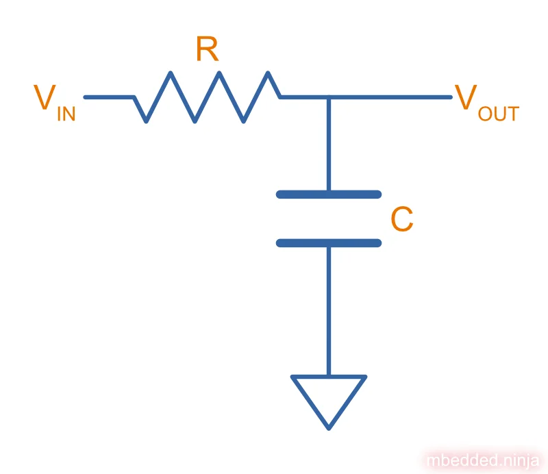
The low-pass RC filter lets through low frequencies but dampens high frequencies.

How To Choose R And C

The cut-off frequency is determined by both the value of the resistor and the value of the capacitor, and is equal to:

$$\begin{align} f_{c} = \frac{1}{2\pi RC} \end{align}$$

where:
\(R\) is the resistance, in Ohms
\(C\) is the capacitance, in Farads
\(f_c\) is the cut-off frequency, in Hertz

As usual, the choice of \(R\) and \(C\) is a design decision which involves trade-offs. In terms of choosing \(R\):

• A resistance which is too small could draw too much current, either presenting too much load to the input, or overheating. It also could mean that the capacitor has to be very large and/or expensive to get the desired cut-off frequency.
• A resistance which is too large increases the output impedance of the filter, resulting in distortions if too much load is applied to \(V_{out}\). It also increases the noise susceptibility of the circuit.

Typically, a resistance between \(1k\Omega\) and \(100k\Omega\) is used. Then the capacitance is chosen to give the desired cut-off frequency.

Frequency Response

To plot the frequency response, we first need to find the transfer function for the low-pass RC filter. We can use the voltage divider rule to write \(v_{out}\) as a function of \(v_{in}\):

$$\begin{align} \frac{V_{out}}{V_{in}} = \frac{X_C}{X_C + R} \end{align}$$

where:
\(v_{in}\) is the magnitude of the input signal at frequency \(f\), in Volts
\(X_C\) is the impedance of the capacitor at frequency \(f\), in Ohms
\(R\) is the resistance of the resistor, in Ohms

Recall that we can write \(X_C\) in the Laplace domain as \(X_C = \frac{1}{sC}\). Also, \(\frac{v_{out}}{v_{in}}\) is just our transfer function \(H(s)\):

$$\begin{align} H(s) = \frac{\frac{1}{sC}}{\frac{1}{sC} + R} \end{align}$$

Multiply top and bottom by \(\frac{1}{sC}\) to clean things up:

$$\begin{align} H(s) = \frac{1}{1 + sRC} \end{align}$$

Now replace \(s\) with \(j\omega\) so we can then take the magnitude:

$$\begin{align} H(j\omega) = \frac{1}{1 + j\omega RC} \end{align}$$

Now take the magnitude (for more info on why and how to do this, see the What Are Transfer Functions, Poles, And Zeroes? page):

$$\begin{align} \label{eq:abc} | H(j\omega) | &= \left| \frac{1}{1 + j\omega RC} \right| \nonumber \\ &= \frac{1}{\sqrt{(1 + j\omega RC)(1 - j\omega RC)}} \nonumber \\ &= \frac{1}{\sqrt{1 - (j\omega RC)^2}} \nonumber \\ &= \frac{1}{\sqrt{1 - (-1)(\omega RC)^2}} \nonumber \\ \label{eq:mag-response-lp-rc-filter} &= \frac{1}{\sqrt{1 + (\omega RC)^2}} \\ \end{align}$$

And let’s find the phase response:

$$\begin{align} \angle H(j\omega) &= Arg\left(H(j\omega)\right) \nonumber \\ &= Arg\left(\frac{1}{1 + j\omega RC}\right) \nonumber \\ &= Arg(1) - Arg(1 + j\omega RC) \nonumber \\ &= 0 - arctan\left(\frac{j\omega RC}{1}\right) \nonumber \\ \label{eq:phase-response-lp-rc-filter} &= -arctan\left(j\omega RC\right) \\ \end{align}$$

This shows us that an RC filter “delays” signals as they pass through. The higher the frequency, the greater the delay.

The following plot shows the frequency response (also known as a bode plot) of a low-pass filter, with values \(R = 1k\Omega\) and \(C = 1\mu F\). Magnitude is plotted in blue and phase in green.

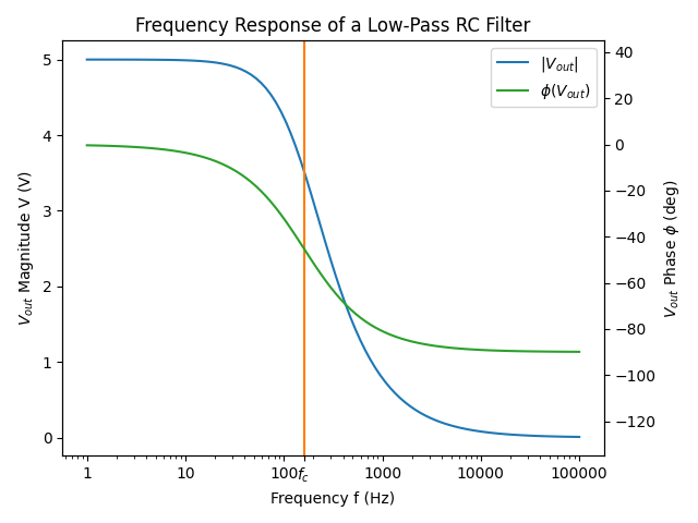
The cut-off frequency (also called the break frequency or turnover frequency¹), \(f_c\) is not the frequency at which all higher frequencies are stopped (remember, this is an ideal filter, but in real-life they always let through some fraction of the higher-frequencies). Instead, it is the frequency at where:

$$\begin{align} V_{out} = \frac{1}{\sqrt{2}} V_{in} = 0.707*V_{in} \end{align}$$

The choice of resistor and capacitor above gives a cut-off frequency of \(f_c = 159Hz\).

Low-pass RC filters are typically used for applications up to 100kHz, above 100kHz RLC filters are used².

Time Constant

The time constant \(\tau\) of a low-pass RC filter is¹:

$$\begin{align} \tau = RC \end{align}$$

Typical Uses

The low-pass RC filter is one (if not) the most commonly used filters on circuit board designs. Its popularity results from it’s simplicity (two passive components), low cost (one resistor, one capacitor), small size, and it’s myriad of uses.

Due to the presence of the resistor, it is a lossy filter, and therefore not suited for high-power applications (use a low-pass LC filter instead).

The low-pass RC filter can be used to provide filtering on analogue inputs to a microcontroller before being sampled by the ADC. One example could be to filter the output of an analogue temperature sensor. Note that is normally advantageous to place the filter as close as possible to the microcontroller, rather than close to the sensor producing the voltage. This is because the series resistor of the RC filter increases the source impedance of the analogue signal, making the PCB track less immune to noise once it passes through the resistor.

Another way to reduce the reduction in noise immunity due to the resistor in the RC low-pass filter is to make the capacitor as large as practically possible (for a particular cut-off frequency). Both the resistance and the capacitance influence the cut-off frequency. If you increase the capacitance by 10x, and reduce the resistance by 10x, you get the same cut-off frequency, but far better noise immunity since the source impedance is not altered as much.

Another consideration is the effect of the increase in source impedance (due to the resistor in the RC filter) when connecting the output to something like a microcontroller ADC). The input impedance of an non-buffered ADC pin on a microcontroller is usually somewhere between \(20-500k\Omega\) (note that this is usually variable, and can change with sampling rate). This will form a resistor divider with the RC filter resistance, increasing the ADC measurement error. As a general rule, you want the RC filter resistance to be much lower than the ADC input impedance.

$$\begin{align} R_{RC filter} << R_{ADC} \end{align}$$

A RC filter resistance which is at least 50x lower than the ADC input impedance is acceptable in most cases. For a standard ADC input impedance of \(50k\Omega\), this means that the resistor in the RC filter should be no more than \(1k\Omega\).

Transient Response

The equation for the voltage across the capacitor is:

$$\begin{align} V_c = V_s(1 - e^{(\frac{t}{RC})}) \end{align}$$

where:
\(V_c\) = voltage across the capacitor, Volts
\(V_s\) = supply voltage, Volts
\(t\) = time since supply was turned on, Seconds
\(R\) = resistance, Ohms
\(C\) = capacitance, Farads

This equation can be re-arranged to find the time \(t\), and which the capacitor is at a certain voltage:

$$\begin{align} t = -log(\frac{V-V_c}{V})RC \end{align}$$

This form of the equation can be useful to calculate the delay (aka the time \(t\)), that the RC circuit will provide before something happens.

Building A VDAC From An ADC And Low-pass RC Filter

Low-pass RC filters can also be used to create a VDAC (voltage-based digital-to-analogue converter) from a PWM signal. This is useful since many microcontrollers have one (or more) PWM peripherals, but rarely a built-in VDAC. A simple RC filter placed on the output pin of the PWM signal can convert it into a VDAC, in where the duty cycle determines the analogue voltage output.

Low-Pass LC Filter

The basic low-pass LC filter consists of a single inductor and capacitor.

Unlike the low-pass RC filter, the low-pass LC filter is theoretically loss-less. This means that it does not dissipate energy as heat. However, real-world inductors have coil resistance and magnetic losses, as well as ESR in the capacitor. Also, the presence of the inductance usually makes the LC filter larger and more expensive than the RC filter.

This makes an LC low-pass filter suitable for higher-power applications. You will see LC low-pass filters being used on the output of buck converters (they are essentially part of the buck converter), to filter the output of an H-bridge, and to filter audio signals before they reach the speakers.

The cut-off frequency of a low-pass LC filter is given by the following equation:

$$\begin{align} f_c = \frac{1}{2\pi \sqrt{LC}} \end{align}$$

The characteristic impedance is:

$$\begin{align} Z = \sqrt{LC} \end{align}$$

which you will notice is also present in the cut-off frequency equation.

Parasitic elements

The main parasitic element to consider with a low-pass LC filter is the parasitic coil resistance of the inductor, \(R_L\). Larger valued inductors typically have a larger coil resistance (due to more windings). This dampens the output signal.

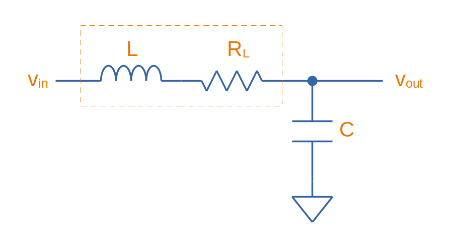
This is equivalent to a low-pass RLC filter.

Low-pass RLC Filter

The quality factor is equal to:

$$\begin{align} Q = \frac{2\pi f}{R} \end{align}$$

As you increase the series resistance, the quality factor decreases.

The damping factor is equal to:

$$\begin{align} d_0 &= \frac{1}{Q} \\ d_0 &= \frac{R}{2\pi fL} \\ \end{align}$$

Low-Pass Pi And t Filters

Low-pass Pi (π) and t-filters are one step better than the low-pass LC or RC filter.

A 1st-order low-pass π-filter has two capacitors and one inductor. The first capacitor absorbs the most AC by shunting it to ground (assuming the input has a finite source impedance). The inductor then blocks remaining AC, allowing only DC to pass through to the second capacitor. The second capacitor then shunts any remaining AC signal back through ground.

The equations for a 1st order filter are:

$$\begin{align} C &= \frac{z_o}{\pi f_c} \\ L &= \frac{1}{z_o \pi f_c} \\ f_c &= \frac{1}{\pi \sqrt{LC}} \\ \end{align}$$

where:
\(C\) = total capacitance in \(F\)
\(L\) = total inductance, in \(H\)
\(z_o\) = characteristic impedance, in \(\Omega\)
\(f_c\) = -3dB cut-off frequency, in \(Hz\)

The typical value to use for the characteristic impedance is \( z_o = 50 \Omega \). Use this if you are unsure on what to set it to. This value is only important if your are matching two RF circuits.

A t-filter is usually better at suppressing high-frequencies than a π-filter, as parasitic coupling between input and output due to PCB layout tends to turn the π filter into a notch filter. However, π-filters are more common because they are cheaper (capacitors are cheaper than inductors).

Both π and t filters may use feedthrough capacitors instead of standard caps for better performance (feedthrough capacitors have lower parasitic series inductance).

Pre-packaged Pi And T Filters

π and t filters can come in pre-packaged components which take all the hassle out of designing the filter correctly and reduce the BOM count of your design. They are commonly in EIAxxxx chip packages.

One such example is the TDK Corporation MEM Series.

2nd-Order Passive Filters

This chaining is also called cascading. The benefit of doing this is that a second-order filter has a roll-off of -40dB/decade, twice that of a first-order filter.

Second-Order Low-Pass RC

The corner frequency \(f_c\) is equal to:

$$\begin{align} f_c = \frac{1}{2\pi \sqrt{R_1 C_1 R_2 C_2}} \end{align}$$

Is is important to remember that for a second-order filter, the gain at the corner frequency is no longer -3dB. Instead it is -6dB. In general, the gain can be described for \(n\) stages with:

$$\begin{align} G = \left( \frac{1}{\sqrt{2}} \right) ^n \end{align}$$

The reduce the effects of each stages dynamic impedance effecting it’s neighbours, its recommended that the following stages resistance should be around 10x the previous stage, and the capacitance 1/10th of the previous stage.

Passive RC Networks With Voltage Gain > 1

It might seem hard to believe, but you can build RC networks which increase the input voltage at specific frequencies. See Herman Epstein - Synthesis Of Passive RC Networks With Gains Greater Than Unity (cached copy, 2021-01-23) for a detailed analysis.

2nd Order Filter Topologies

A filter topology is an actual circuit configuration which can realize a number of different filter designs. This is different from the configurations such as Butterworth, Chebyshev and Bessel which define the component tuning

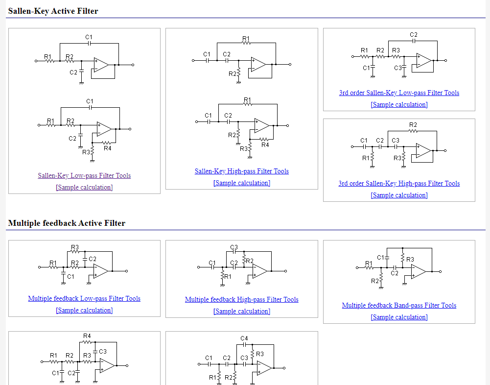
• Sallen-Key (a.k.a. KRC filters)
• Tow-Thomas
• Multiple-Feedback Filters (a.k.a. infinite-gain filters)
• State-Variable Filters: As known as KHN filters after the inventors W. J. Kerwin, L. P. Huelsman and R. W. Newcomb, first reported in 1967³.

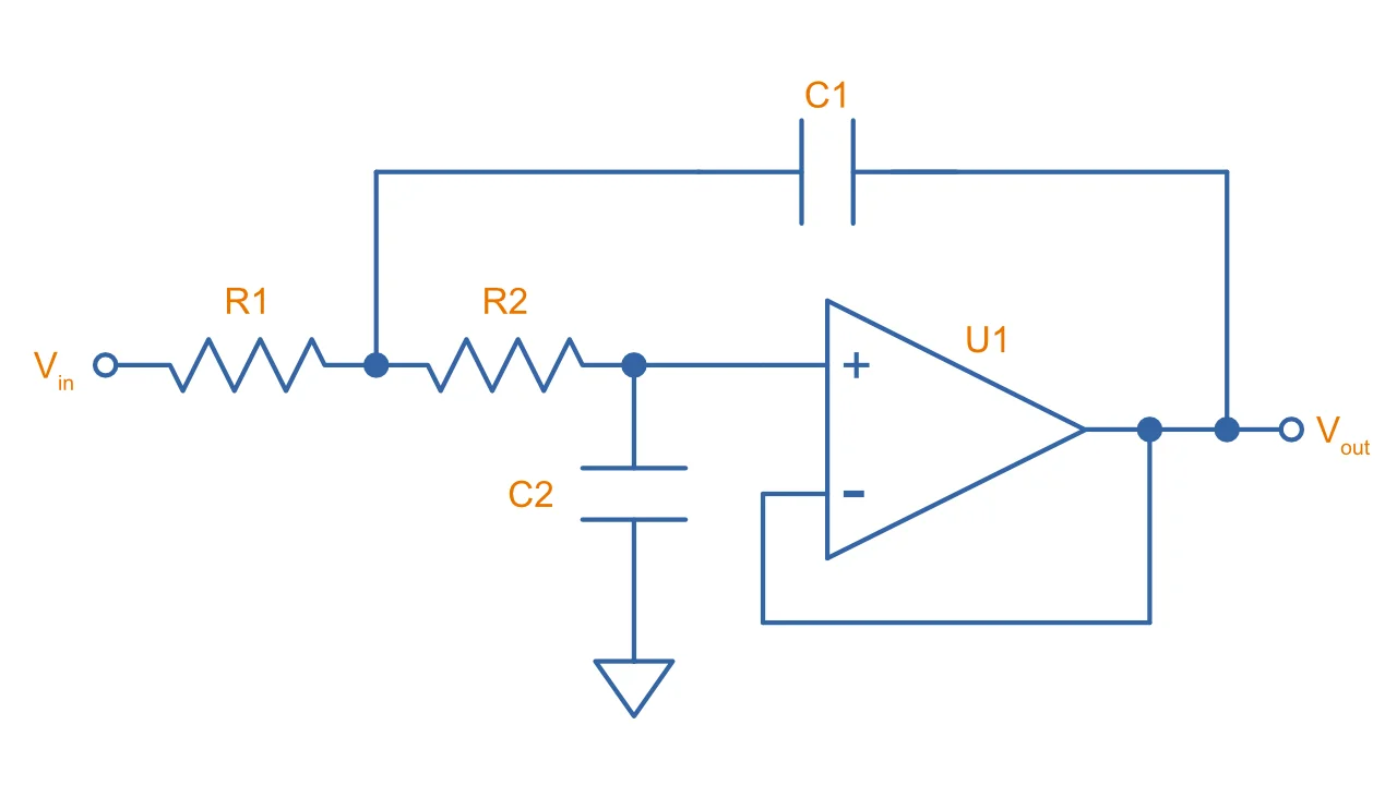
Voltage-Controlled Voltage-Source (VCVS) Filters

Voltage-controlled voltage-source (VCVS) filters are an extension of the Sallen-Key filter (in that sense, the Sallen-Key filter can be thought of as a simplification of the VCVS filter in where the voltage gain of the op-amp is set to one) in where standard resistor divider feedback is added between the op-amp’s output and the inverting input, allowing the gain of the filter to be something other than \(1\).

They are called VCVS filters because the op-amp is used as a voltage amplifier.

Design Tools

OKAWA Filter Design and Analysis

Website: http://sim.okawa-denshi.jp/en/Fkeisan.htm

Great site with web-based calculators and design tools for active and passive filters. Very detailed site with many configuration options and the site even outputs graphs of your designed filter response.

PSoC Microcontrollers And The PSoC Creator IDE

The PSoC microcontroller features an in-built and versatile digital filter block, and the IDE has a graphically-edited method of configuring the DFB to do exactly what you want. The IDE even shows you graphs of the expected response (magnitude, phase, step plots e.t.c).

External Resources

• The New Jersey Institute of Technology EE 494 Laboratory IV Part B lab manual is a great practical resource for learning how to design active filters.
• The Design With Operational Amplifiers And Analog Integrated Circuits by Sergio Franco, Fourth Edition is a great book to purchase if you are interesting in further reading and getting right into the weeds of analogue filter design!
• Op Amps For Everyone by Ron Mancini (SLOD006B) has some detailed sections on op-amp filter circuits.
• SLOA024B: Analysis of the Sallen-Key Architecture - Application Report, by Texas Instruments can be used for further reading on the Sallen-Key and VCVS amplifiers (cached local copy).
• Texas Instruments Filter Designer is a free online tool to design filters.
• The Analog Devices Filter Wizard is an alternative to the Texas Instruments version.

References