Chirps

Caution

This page is in notes format, and may not be of the same quality as other pages on this site.

A chirp is a signal whose frequency changes over time. Up chirps are signals whose frequency increases over time, and down chirps are signals whose frequency decreases over time. The frequency change can be linear (if the rate of change is not mentioned, it can be assumed to be linear), exponential, or some other function.

Chirps are present in many natural and man-made systems. Animals such as birds, frogs and whales create audible chirps, and bats use chirps in the ultrasonic range for echolocation. Chirps are also present in music (“glissando”).¹

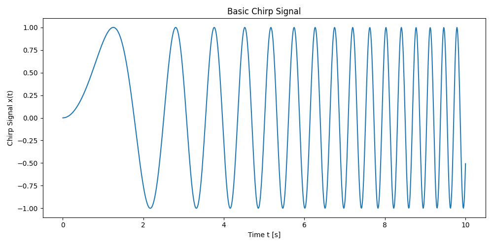
The simplest chirp signal can be created by squaring the time variable in a normal sinusoidal signal, for example:

$$\begin{align} x(t) = \sin(t^2) \end{align}$$

This is a placeholder for the reference: fig-basic-chirp-signal shows a plot of this basic chirp signal.

A plot showing a basic chirp signal using the equation $x(t) = \sin(t^2)$.

Chirp signals are often used in radar and communication systems due to their favourable properties, such as constant amplitude, good autocorrelation properties, and resistance to Doppler shifts. The low power RF communication protocol LoRa uses chirp signals (specifically, a proprietary form of chirp spread spectrum where each symbol has a different starting frequency) to encode information.²

Basic Equations

These basic equations are applicable to most chirp signals including the linear chirps. These equations will be used in the following sections as needed.

A chirp signal $x(t)$ can be described by the following equation:

$$\begin{align} x(t) = \sin(\phi(t)) \end{align}$$

where:
$x(t)$ is the chirp signal at time $t$
$\phi(t)$ is the phase at time $t$, in $rad$

Angular frequency $\omega(t)$ is the rate of change of phase $\phi(t)$. Thus:

$$\begin{align} \omega(t) = \frac{d\phi(t)}{dt} \end{align}$$

Rewriting this in terms of $\phi(t)$ gives:

$$\begin{align} \phi(t) = \phi_0 + \int_0^t \omega(\tau) d\tau \end{align}$$

where:
$\phi_0$ is the initial phase at time $t = 0$, in $rad$ (we need to add this because the definite integral only gives us the change in phase from 0 to $t$, not the absolute phase at time $t$)

Note

What’s this new $\tau$ (tau) variable, and how is it different from $t$? $\tau$ is a dummy variable of integration. $t$ is the specific moment in which you want to know $\phi(t)$, while $\tau$ is a placeholder which “sweeps” through all times from $0$ up to $t$ as part of the integration.

And since $\omega(t) = 2\pi f(t)$, we can write:

$$\begin{align} \phi(t) = \phi_0 + 2\pi \int_0^t f(\tau) d\tau \end{align}$$

This equation will be useful to convert from frequency to phase so that we can create the equation for the chirp signal $x(t)$.

Linear Chirps

A linear chirp is a chirp in which the frequency changes linearly over time. Thus:³

$$\begin{align} f(t) = ct + f_0 \end{align}$$

where:
$f(t)$ is the frequency at time $t$, in $Hz$
$f_0$ is the starting frequency at time $t = 0$, in $Hz$
$c$ is the rate of change of frequency, in $Hz/s$
$t$ is the time, in $s$

The phase equation $\phi(t)$ for any oscillating signal is always the integral of the frequency function $f(t)$.

$$\begin{align} \phi(t) &= \phi_0 + 2\pi \int_0^t f(\tau) d\tau \nonumber \\ &= \phi_0 + 2\pi \int_0^t (f_0 + c\tau) d\tau \nonumber \\ &= \phi_0 + 2\pi \left( \frac{c}{2}t^2 + f_0t \right) \\ \end{align}$$

Now that we have the phase equation, we can write the equation for the linear chirp signal as (since $x(t) = \sin(\phi(t))$):

$$\begin{align} x(t) &= \sin(\phi(t)) \nonumber \\ &= \sin\left( \phi_0 + 2\pi \left[ \frac{c}{2}t^2 + f_0t \right] \right) \\ \end{align}$$

where:
$\phi_0$ is the starting phase at time $t = 0$, in $rad$

Example

Let’s create a linear chirp with the following parameters:

• Starting frequency: $f_0 = 1\ \text{kHz}$
• Rate of change of frequency: $c = 100\ \text{kHzs}^{-1}$
• Initial phase: $\phi_0 = 0\ \text{rad}$

This would give us the following equation for the signal $x(t)$:

$$\begin{align} x(t) &= \sin\left( 0 + 2\pi \left[ \frac{100 \text{kHzs}^{-1}}{2}t^2 + 1 \text{kHz} \cdot t \right] \right) \nonumber \\ &= \sin\left( 2\pi \left[ 50\text{kHzs}^{-1} \cdot t^2 + 1\text{kHz} \cdot t \right] \right) \\ \end{align}$$

This is a placeholder for the reference: fig-linear-chirp-signal shows a plot of this linear chirp signal for the first 20 milliseconds.

A plot showing a linear chirp signal using the equation $x(t) = \sin\left( 2\pi \left[ 50\text{kHzs}^{-1} \cdot t^2 + 1\text{kHz} \cdot t \right] \right)$.

This is a placeholder for the reference: fig-linear-chirp-spectrogram shows a spectrogram of the same linear chirp signal. A spectrogram displays how the frequency content of a signal changes over time, with time on the horizontal axis, frequency on the vertical axis, and power spectral density shown as color intensity. The linear increase in frequency over time is clearly visible as a diagonal line from 1 kHz at $t = 0$ to 3 kHz at $t = 20\ \text{ms}$.

A spectrogram showing the frequency content of the linear chirp signal over time. The diagonal line shows the linear increase in frequency from 1 kHz to 3 kHz over 20 milliseconds. The signal was sampled at 100 kHz. Each spectrogram window (bin) contains 512 samples (5.12ms @ 100 kHz). The signal was padded at the beginning and end (with an extrapolated chirp signal, not just zeros) to there was no blank areas on the left and right.

Exponential Chirps

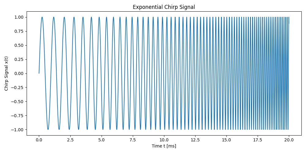
An exponential chirp (also called a geometric chirp) is a chirp in which the frequency changes exponentially over time. This means for any two points in time $t_1$ and $t_2$ where the time interval $T (\Delta t = t_2 - t_1)$ is kept constant, the frequency ratio $\frac{f(t_2)}{f(t_1)}$ is also kept constant.

This is a placeholder for the reference: fig-exponential-chirp-signal shows a plot of an exponential chirp signal.

A plot showing an exponential chirp signal. This chirp starts at 1 kHz and exponentially increases to 8 kHz after 20 milliseconds.

The frequency $f(t)$ of an exponential chirp is given by the following equation:³

$$\begin{align} f(t) = f_0 k^{\frac{t}{T}} \end{align}$$

where:
$f(t)$ is the frequency at time $t$, in $Hz$
$f_0$ is the initial frequency at time $t = 0$, in $Hz$
$k$ is the frequency ratio, a constant
$T$ is the time interval between the two points in time, in $s$

The frequency ratio $k$ is given by the following equation:

$$\begin{align} k = \frac{f_1}{f_0} \end{align}$$

where:
$f_1$ is the frequency at time $t_1$, in $Hz$
$f_0$ is the initial frequency at time $t = 0$, in $Hz$

We can write the phase equation $\phi(t)$ by integrating the frequency equation:

$$\begin{align} \phi(t) &= \phi_0 + 2\pi \int_0^t f(\tau) d\tau \nonumber \\ &= \phi_0 + 2\pi \int_0^t f_0 k^{\frac{\tau}{T}} d\tau \nonumber \\ &= \phi_0 + 2\pi f_0 \left[ \frac{T(k^\frac{t}{T} - 1)}{ln(k)} \right] \end{align}$$

To get the equation for the exponential chirp signal $x(t)$, we substitute this equation for phase into $x(t) = \sin(\phi(t))$.

$$\begin{align} x(t) &= \sin(\phi(t)) \nonumber \\ &= \sin\left( \phi_0 + 2\pi f_0 \left[ \frac{T(k^\frac{t}{T} - 1)}{ln(k)} \right] \right) \end{align}$$

Example

Let’s create an exponential chirp with the following parameters:

• Initial frequency: $f_0 = 1\ \text{kHz}$
• End frequency: $f_1 = 8\ \text{kHz}$ (this gives a frequency ratio $k = \frac{f_1}{f_0} = 8$)
• Time interval: $T = 20\ \text{ms}$
• Initial phase: $\phi_0 = 0\ \text{rad}$

This would give us the following equation for the signal $x(t)$:

$$\begin{align} x(t) &= \sin\left( 0 + 2\pi \left[ \frac{20\ \text{ms}(8^\frac{t}{20\ \text{ms}} - 1)}{ln(8)} \right] \right) \nonumber \\ &= \sin\left( 2\pi \left[ \frac{20\ \text{ms}(8^\frac{t}{20\ \text{ms}} - 1)}{ln(8)} \right] \right) \\ \end{align}$$

If we plot this, we get the waveform shown in This is a placeholder for the reference: fig-example-exponential-chirp-signal.

A plot showing an exponential chirp signal using the equation $x(t) = \sin\left( 2\pi \left[ \frac{20\ \text{ms}(8^\frac{t}{20\ \text{ms}} - 1)}{ln(8)} \right] \right)$.

This is a placeholder for the reference: fig-example-exponential-chirp-spectrogram shows a spectrogram of the same exponential chirp signal.

A spectrogram showing the frequency content of the exponential chirp signal over time. The signal was sampled at 500 kHz. Each spectrogram window (bin) contains 2048 samples (4.096ms @ 500 kHz). The signal was padded at the beginning and end (with an extrapolated chirp signal, not just zeros) to there was no blank areas on the left and right.

Hyperbolic Chirps

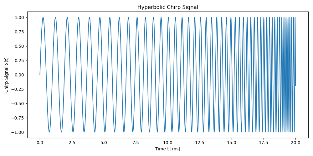
Hyperbolic chirps are used in radar and wideband active sonar systems as a way of minimizing degradation of matched filter processing when the source and target are moving with respect to each other.^{4 3}

Tip

A matched filter is when you look for the sent signal in the received signal. You do this by correlating the received signal with the sent signal. You will get a sharp peak in the correlation when the signals correlate, telling you a reflection has been received.

Hyperbolic chirps correlate well with the original signal even after being doppler shifted. See the Doppler Tolerance and Matched Filter Performance section for more details.

This is a placeholder for the reference: fig-hyperbolic-chirp-signal shows a plot of a hyperbolic chirp signal.

A plot showing a hyperbolic chirp signal. This chirp starts at 1 kHz and hyperbolically increases to 8 kHz after 20 milliseconds.

The frequency $f(t)$ of a hyperbolic chirp is given by the following equation:³

$$\begin{align} f(t) = \frac{f_0 f_1 T}{(f_0 - f_1)t + f_1 T} \end{align}$$

where:
$f(t)$ is the frequency at time $t$, in $Hz$
$f_0$ is the initial frequency at time $t = 0$, in $Hz$
$f_1$ is the final frequency at time $t = T$, in $Hz$
$T$ is the time interval between the two points in time, in $s$

We can integrate the frequency equation to get the phase equation $\phi(t)$:³

$$\begin{align} \phi(t) &= \phi_0 + 2\pi \int_0^t f(\tau) d\tau \nonumber \\ &= \phi_0 + 2\pi \int_0^t \frac{f_0 f_1 T}{(f_0 - f_1)\tau + f_1 T} d\tau \nonumber \\ &= \phi_0 + 2\pi \frac{-f_0 f_1 T}{f_1 - f_0} \ln \left( 1 - \frac{f_1 - f_0}{f_1 T}t \right) \end{align}$$

where:
$\phi(t)$ is the phase at time $t$, in $rad$
$\phi_0$ is the initial phase at time $t = 0$, in $rad$

To get the equation for the hyperbolic chirp signal $x(t)$, we substitute this equation for phase into $x(t) = \sin(\phi(t))$.

$$\begin{align} x(t) &= \sin(\phi(t)) \nonumber \\ &= \sin\left( \phi_0 + 2\pi \frac{-f_0 f_1 T}{f_1 - f_0} \ln \left( 1 - \frac{f_1 - f_0}{f_1 T}t \right) \right) \end{align}$$

Example

Let’s create a hyperbolic chirp with the following parameters:

• Initial frequency: $f_0 = 1\ \text{kHz}$
• End frequency: $f_1 = 8\ \text{kHz}$
• Time interval: $T = 20\ \text{ms}$
• Initial phase: $\phi_0 = 0\ \text{rad}$

This would give us the following equation for the signal $x(t)$:

$$\begin{align} x(t) &= \sin\left( 0 + 2\pi \frac{-1\ \text{kHz} \cdot 8\ \text{kHz} \cdot 20\ \text{ms}}{8\ \text{kHz} - 1\ \text{kHz}} \ln \left( 1 - \frac{8\ \text{kHz} - 1\ \text{kHz}}{8\ \text{kHz} \cdot 20\ \text{ms}}t \right) \right) \nonumber \\ &= \sin\left( -143.62 \ln (1 - 43.75 t) \right) \end{align}$$

If we plot this, we get the waveform shown in This is a placeholder for the reference: fig-example-hyperbolic-chirp-signal.

A plot showing a hyperbolic chirp signal using the equation $x(t) = \sin\left( -143.62 \ln (1 - 43.75 t) \right)$.

This is a placeholder for the reference: fig-example-hyperbolic-chirp-spectrogram shows a spectrogram of the same hyperbolic chirp signal.

A spectrogram showing the frequency content of the hyperbolic chirp signal over time. The signal was sampled at 500 kHz. Each spectrogram window (bin) contains 2048 samples (4.096ms @ 500 kHz). The signal was padded with extrapolated values at the start, but with zeroes at the end due to the inability to calculate $\ln$ for negative numbers.

Doppler Tolerance and Matched Filter Performance

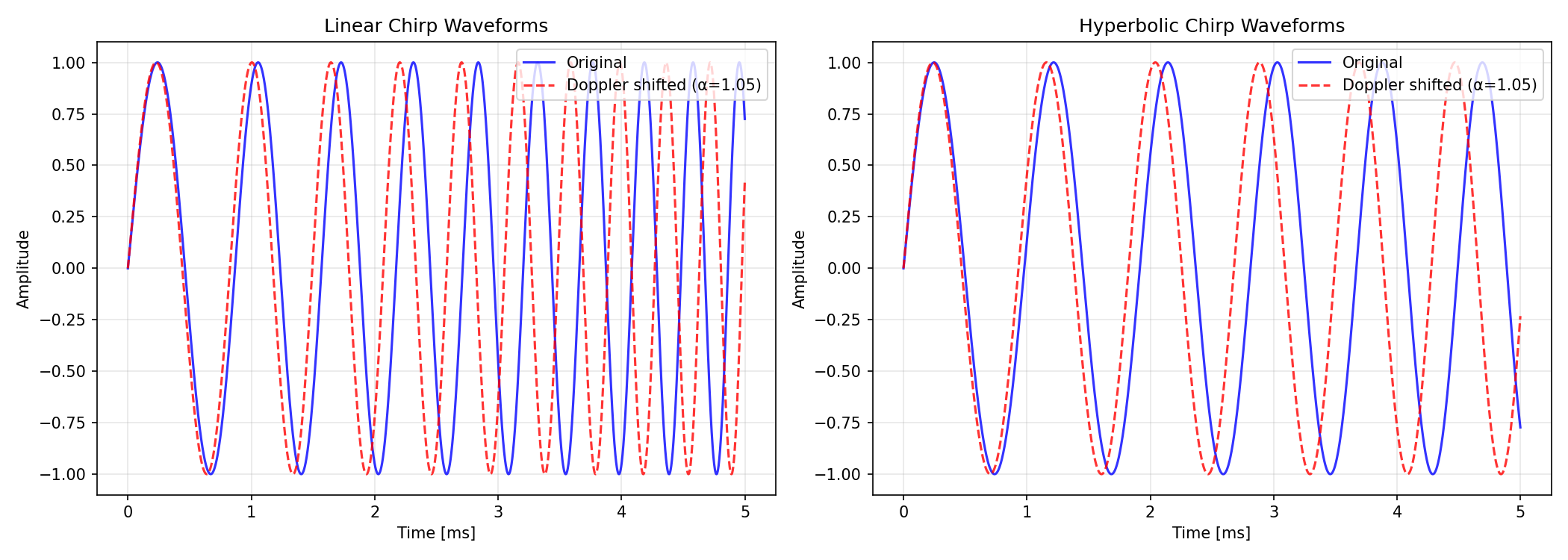
One of the most important properties of hyperbolic chirps is their Doppler tolerance. In radar and sonar systems, when a signal reflects off a moving target, the received signal undergoes a Doppler shift. This shift not only changes the frequency content but also compresses or stretches the signal in time.

Mathematically, if the transmitted signal is $s(t)$, the received signal from a moving target is:

$$\begin{align} r(t) = s(\alpha t) \end{align}$$

where:
$\alpha$ is the time-scaling factor due to Doppler effect

For a two-way propagation system (a.k.a. pulse-echo — like active sonar or radar), the time-scaling factor $\alpha$ is given by the following equation:

$$\begin{align} \alpha = 1 + \frac{2v}{c} \end{align}$$

where:
$\alpha$ is the time-scaling factor due to Doppler effect
$v$ is the relative velocity between source and target, in $m/s$
$c$ is the speed of wave propagation (speed of light for radar, speed of sound for sonar), in $m/s$

The factor of 2 in the above equation comes from the fact it is a round-trip (the signal gets distorted on the way out and back).

Note

The Doppler effect is much more significant in sonar than radar because sound travels ~200,000x slower than light in air. A 37 m/s target produces $\alpha \approx 1.05$ in sonar but only $\alpha \approx 1.00000025$ in radar.

This is a placeholder for the reference: fig-doppler-waveform-comparison shows a side-by-side comparison of the original and Doppler-shifted waveforms. This zooms into the first 5 milliseconds to show the difference more clearly.

Side-by-side comparison of the original and Doppler-shifted waveforms.

A matched filter is a signal processing technique where the received signal is correlated with a copy of the transmitted signal to detect the presence and timing of echoes. The output produces a sharp peak when the signals align, indicating a detection.

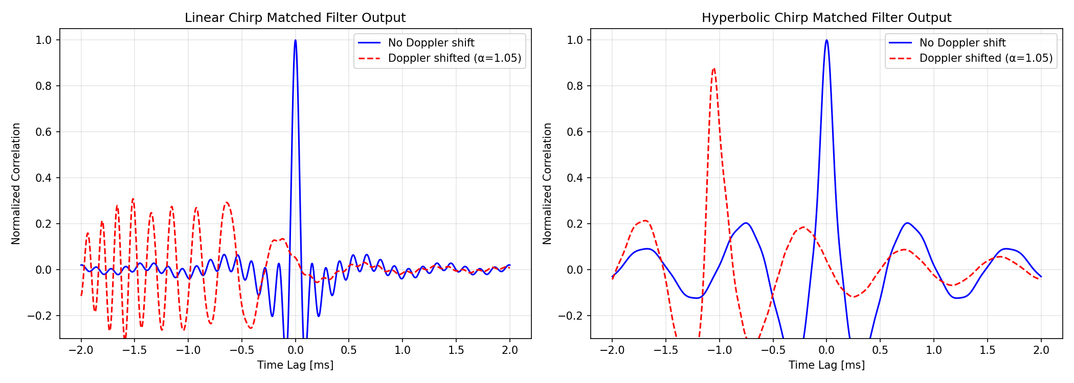
The key problem is that when the received signal is doppler shifted, it gets scaled with respect to time. For linear chirps, this means that the received signal will only match the original signal at a single instant, as the received signal is sweeping through frequencies at a faster/slower rate. This means the correlation peak will be:

• Reduced in peak amplitude (harder to detect)
• Spread out in time (reduced range resolution)

Hyperbolic chirps have a special property: when time-scaled, they are equivalent to a time-shifted version of the original signal. This means the Doppler-shifted signal still correlates well with the original (just with a shifted started point), maintaining a sharp peak in the matched filter output.

This is a placeholder for the reference: fig-doppler-matched-filter-comparison shows a side-by-side comparison of matched filter outputs for linear and hyperbolic chirps, both with and without Doppler shift ($\alpha = 1.05$, representing approximately 5% time compression). The negative time lag for the peaks in the doppler shifted waveforms is due to the signal being compressed in time — the received signal “finishes early” and the correlation maximum shift to where the compressed signal best aligns with the original.

Side-by-side comparison of matched filter outputs for linear (left) and hyperbolic (right) chirps. The blue solid line shows the ideal case with no Doppler shift, while the red dashed line shows the response when the received signal is Doppler-shifted by $\alpha = 1.05$. Notice how the linear chirp’s peak is significantly reduced and broadened, while the hyperbolic chirp maintains a much sharper peak.

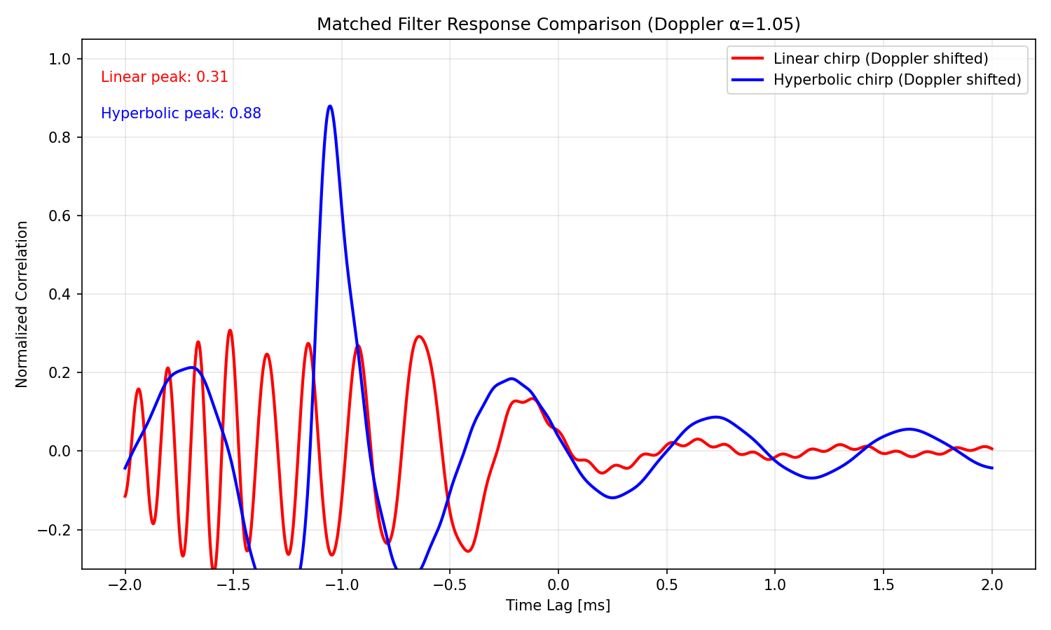
This is a placeholder for the reference: fig-doppler-tolerance-overlay provides a direct overlay comparison of just the Doppler-shifted responses, making the difference even clearer. The linear chirps correlation peak only hits a peak normalized correlation value of 0.31, whilst the hyperbolic chirp hits a peak of 0.88!

Direct comparison of matched filter responses for Doppler-shifted linear and hyperbolic chirps ($\alpha = 1.05$). The hyperbolic chirp maintains a significantly higher and sharper correlation peak compared to the linear chirp, demonstrating its superior Doppler tolerance.

Footnotes

1. Patrick Flandrin. Time-frequency and chirps. Ecole Normale Superieure de Lyon. Retrieved 2026-01-14, from https://perso.ens-lyon.fr/patrick.flandrin/SPIE01_PF.pdf. ↩

2. Wikipedia (2025, Dec 10). LoRa [wiki]. Retrieved 2026-01-04, from https://en.wikipedia.org/wiki/LoRa. ↩

3. Wikipedia (2025, Sep 3). Chirp [wiki]. Retrieved 2026-01-12, from https://en.wikipedia.org/wiki/Chirp. ↩ ↩² ↩³ ↩⁴ ↩⁵

4. Mark Readhead. Calculations of the Sound Scattering of Hyperbolic Frequency Modulated Chirped Pulses from Fluid-filled Spherical Shell Sonar Targets. Australian Department of Defence. Retrieved 2026-01-14, from https://apps.dtic.mil/sti/pdfs/ADA523424.pdf. ↩