Analytic Signal

An analytic signal is a complex-valued function that has no negative frequency components. It is created by taking the Hilbert transform of a real-valued function and then adding the original function with the imaginary number multiplied by the Hilbert transform.

The analytic signal is useful in signal processing because it can be used to calculate various features of a signal at different points in time, such as the instantaneous amplitude, frequency and phase of a signal. It can aid in the demodulation of amplitude modulated signals.

Calculation

One way to calculate the analytic signal $s_a(t)$ of a real-valued function $s(t)$ is:

$$\begin{align} s_a(t) = s(t) + j\ \text{Hilbert}(s(t)) \end{align}$$

where:
$s_a(t)$ is the computed analytic signal
$s(t)$ is the original real-valued function
$j$ is the imaginary number ($j = \sqrt{-1}$), also seen as $i$ in maths ($j$ is used in electronics as to not get $i$ confused with current)
$\text{Hilbert}(s(t))$ is the Hilbert transform of $s(t)$

Because we enforce the condition that the original function be real-valued (i.e. have no imaginary components), you can easily go backwards from the analytic signal to the original real-valued function by discarding the imaginary part.

The above equation is in the time domain. You can also calculate the analytic signal in the frequency domain $S_a(f)$ using the following equation:

$$\begin{align} S_a(f) = 2u(f)S(f) \end{align}$$

where:
$S_a(f)$ is the computed analytic signal in the frequency domain
$S(f)$ is the original real-valued function in the frequency domain
$u(f)$ is the Heaviside step function

This equation shows that, in the frequency domain, the analytic signal is calculated simply by:

1. Removing all the negative frequency components
2. Doubling the magnitude of the positive frequency components

Instantaneous Amplitude, Frequency and Phase

One thing the analytic signal is useful for is finding the instantaneous amplitude, frequency and phase of a signal.

Tip

It’s important to understand that “instantaneous” refers to the concept that, at any specific point of time, you can characterise the signal by a single amplitude, frequency and phase. This only works well for narrowband signals — signals in where all the energy is concentrated in a narrow band of frequencies. This is true for AM modulated signals in where all the energy is concentrated around the carrier frequency.¹

The instantaneous amplitude $s_m(t)$ is found by taking the magnitude of the analytic signal (remembering that the analytic signal is a complex number and the magnitude is the distance from the origin to the complex number on the complex plane):

$$\begin{align} s_m(t) = |s_a(t)| \end{align}$$

The instantaneous phase $\theta(t)$ of the signal is found by taking the argument of the analytic signal (remembering that the analytic signal is a complex number, and the argument is the angle from the positive x-axis to the line connecting the origin to the complex number on the complex plane):²

$$\begin{align} \theta(t) = \arg [s_a(t)] \end{align}$$

The instantaneous angular frequency $\omega(t)$ of the signal is found by taking the derivative of the unwrapped instantaneous phase with respect to time (i.e. it is the rate of change of phase):²

$$\begin{align} \omega(t) = \frac{d}{dt} \theta(t) \end{align}$$

Converting from angular frequency to Hertz gives us the instantaneous frequency $f(t)$:²

$$\begin{align} f(t) = \frac{1}{2\pi} \omega(t) \end{align}$$

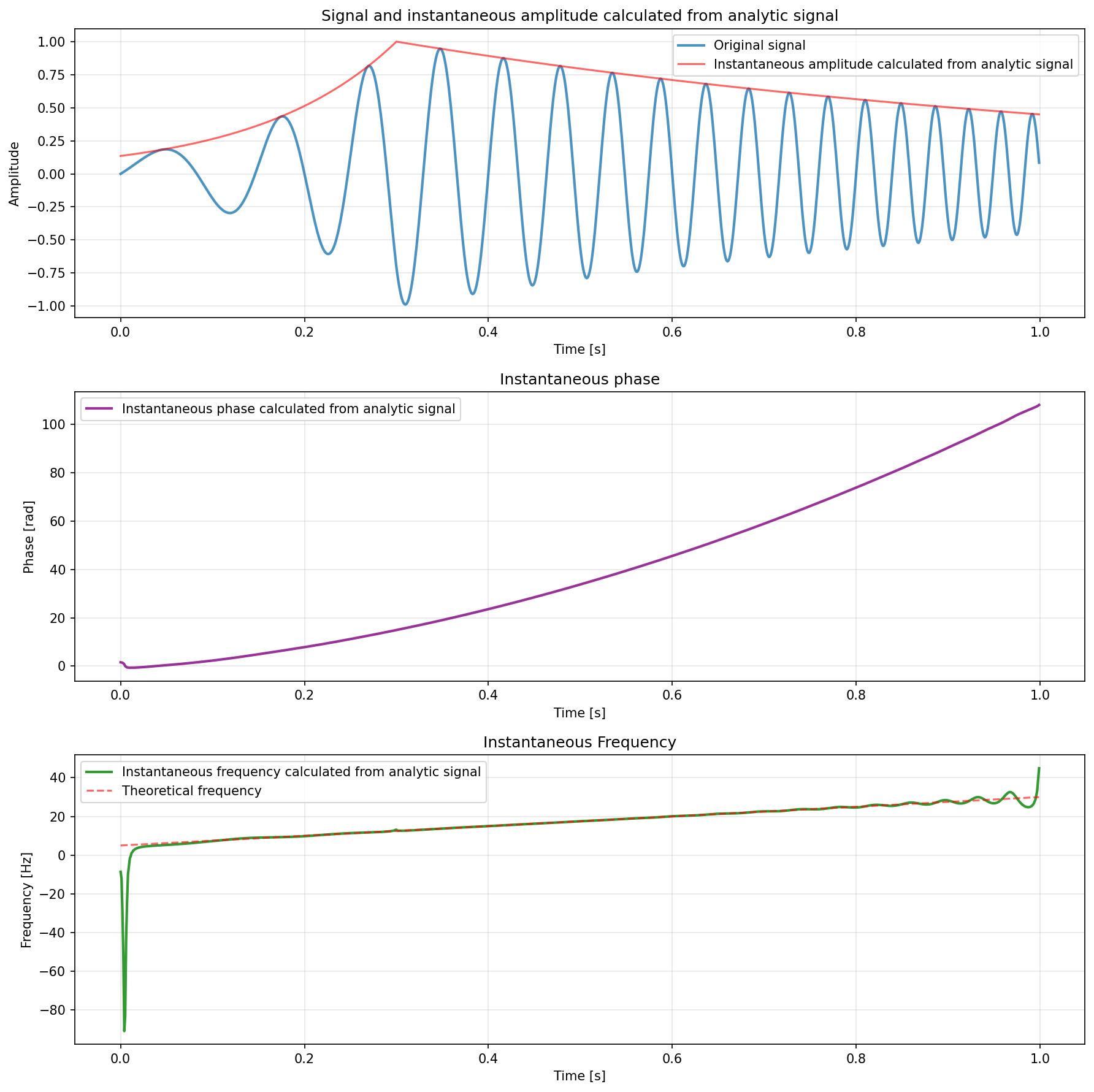
This is a placeholder for the reference: fig-chirp-and-analytic-signal shows a frequency and amplitude changing signal (commonly known as a chirp) and its analytic signal. The signal I created for analysis was a chirp which starts at 5 Hz and linearly ramps to 30 Hz over 1 second. The amplitude of the chirp is also varying. It first begins to exponentially rise until $t = 0.3 s$, and then exponentially falls at a slower rate until the end.

You can see how the instantaneous amplitude calculated from the analytic signal closely follows the original amplitude envelope and how it can be a useful way to demodulate amplitude modulated signals. Also useful is the calculated instantaneous phase and frequency. Note how the calculated instantaneous frequency closely matches the theoretical frequency is used to create the chirp in the first place, except for just after $t = 0 s$.

Time domain and frequency domain plots of a frequency and amplitude changing signal (commonly known as a chirp) and its analytic signal.

When Instantaneous Frequency Doesn’t Work Well

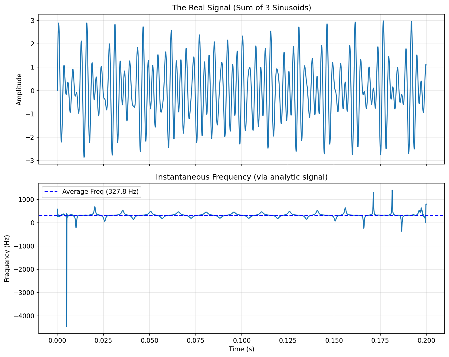
Calculating the instantaneous frequency does not work well with wideband signals. Let’s take a look at an example. Let’s make a signal of a C major triad from three sine waves at 261.63 Hz, 329.63 Hz and 392.00 Hz (C4 — middle C, E4, G4). Then let’s calculate the analytic signal and the instantaneous frequency. This is a placeholder for the reference: fig-widely-varying-instantaneous-frequency shows the results. Note how the calculated instantaneous frequency jumps all over the place, including going down to -4000 Hz! This is due to destructive interference between the three sine waves causing the amplitude of the signal to go close to zero at certain points in time. At these times, small movements can cause large changes in the angle in the complex plane (large phase changes) resulting in large changes in the instantaneous frequency (which is the derivative of the phase).

Time domain and frequency domain plots of a signal with widely varying instantaneous frequency.

Python

The Python library SciPy provides the scipy.signal.hilbert() function to compute the analytic function of a signal.³

Tip

scipy.signal.hilbert() is named confusingly. It actually returns the analytic signal, not just the Hilbert transform. If you just wanted the Hilbert transform, you need to take the imaginary part of the returned analytic signal, which is np.imag(scipy.signal.hilbert(signal)) (assuming you are using NumPy).³

Footnotes

1. Julius O. Smith III (2024, Apr 2). Analytic Signals and Hilbert Transform Filters. Stanford University. Retrieved 2025-12-17, from https://ccrma.stanford.edu/~jos/st/Analytic_Signals_Hilbert_Transform.html. ↩

2. Wikipedia (2025, Sep 18). Analytic signal. Retrieved 2025-12-16, from https://en.wikipedia.org/wiki/Analytic_signal. ↩ ↩² ↩³

3. SciPy. SciPy API > Signal processing (scipy.signal) > hilbert. Retrieved 2025-12-17, from https://docs.scipy.org/doc/scipy/reference/generated/scipy.signal.hilbert.html. ↩ ↩²