Capacitor Encoder Design

This page describes how to design a capacitor encoder with just two PCBs with cleverly etched tracks, a capacitance-to-digital converter IC, and a microcontroller with some signal processing/algorithm code.

Terminology

Caution

This is my terminology, and may not be consistent with other designs (as far as I’m aware, there is no industry standard).

• Encoders: A encoder is a complete system which can be used to measure a position. It may have one (relative) or more (two for absolute) tracks.
• Tracks: A sequence of capacitance pads and tracks used for measuring the position of an object. One or more of these make up a complete encoder. A track contains many channels.
• Channels: A channel is a single electrical circuit in which the capacitance can be measured. A track consists of many channels (e.g. 6). The channels capacitance varies as the PCBs slide across one another.
• Signature Waveform: The expected shape of the waveform made when you group together the capacitance channels for a track. The measured capacitance values are made into an array and the compared with the signature waveform by calculating the correlation coefficient.

How They Work

The basic principle is two PCBs, which slide across each other. The PCBs have multiple specially shaped copper areas, and the capacitance between the copper areas on each PCB change as the PCBs move. The capacitances are measured with a CDC (capacitance-to-digital converter), and then a signal processing algorithm is used to determine one PCBs position relative to the other.

What You Will Need

• PCBs with etched “pads” and “finger”, more on this later
• A capacitance-to-digital converter (CDC)
• A microcontroller
• A suitable dielectric

The microcontroller needs to have enough memory and processing speed to do a bit of signal processing. I’m not talking intense DSP or FPGA levels of signal processing, but there is enough of it that it does rule out most lower end microcontrollers. I would recommend a 32-bit micro with at least 64kB of flash and 8kB of RAM, with a clock speed >24MHz, for processing one absolute capacitive encoder.

What Resolution/Accuracy Is Possible?

I have achieved resolutions of up to 4/100 of a degree with custom-built absolute rotational capacitance encoders, which is equivalent to a 9000 count/rev encoder! The accuracy of these measurements was never calculated, although I suspect it would be high.

What limits the resolution/accuracy?

(approx. in order of importance)

• Number of active pads per electrical period
• The electrical period (aka size of the passive pad)
• Capacitance measuring (CDC) accuracy
• Processor speed
• Number of capacitive channels to measure
• PCB manufacturing tolerances

PCB Design

Soldermask must be applied to all parts of both tracks which are rubbing against each other. You want the circuit to be capacitively coupled, not a direct short. The soldermask acts as a dielectric (but more dielectric material should be added, see below).

What PCB Is Active And What Is Passive

• The PCB with the cap measuring circuitry (requiring power) is Active.
• The PCB with only etched tracks is Passive.

Altium Script

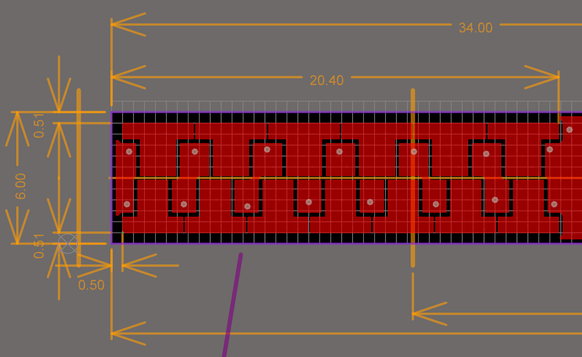
I wrote an Altium script to draw the tracks for me. Although you could do it by hand (a linear one would be of medium difficulty to draw manually, a rotational one would be even harder, even with the rotational co-ordinate functionality in Altium).

The Altium script takes input variables such as N track length, number of passive pads in the N track, number of active fingers per wavelength, desired total width, minimum copper clearance e.t.c and using plenty of trigonometry, creates the tracks automatically, saving tons of time!

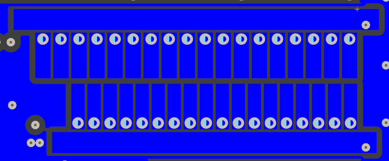
Linear

A linear capacitive encoder passive PCB.

A linear capacitive encoder active PCB.

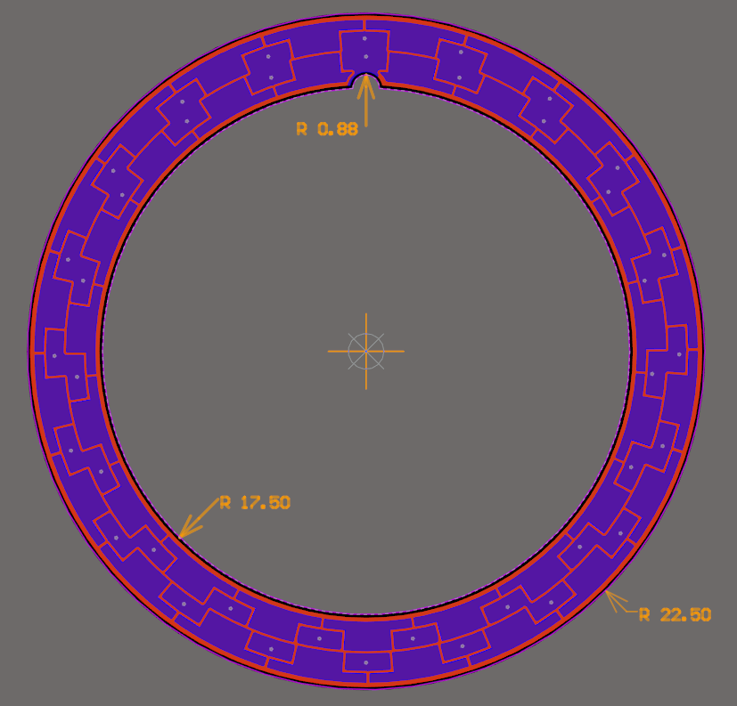
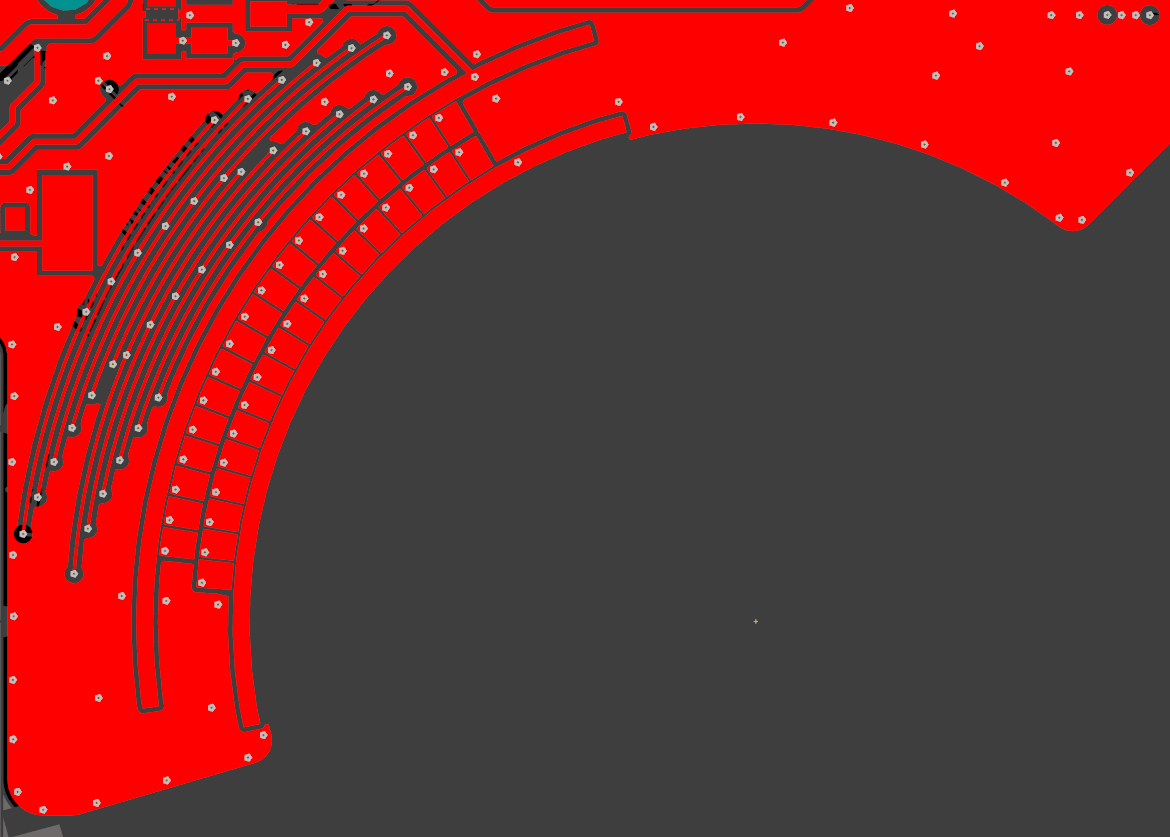
Rotational

A rotational capacitive encoder design is very much like the linear one, except everything is drawn on polar co-ordinate system rather than a cartesian. The biggest difference is that the rotational one can be continuous (i.e. the tracks can rotate a full 360, and there is no stop or end point).

A rotational capacitive encoder passive PCB.

A rotational capacitive encoder active PCB.

The Dielectric

I recommend adding a dielectric between the PCBs (as well as the soldermask). Counter-intuitively, any dielectric added decreases the total capacitance. This is because although the dielectric increases the dielectric constant, it also increases the distance between the plates. This distance increase as a bigger effect on the capacitance than the dielectric increase, as per the parallel-plate equation on the Capacitors page.

The reason I recommend adding a dielectric is that it stabilizes the capacitances. It reduces the change in capacitance due to the two PCBs moving away from each other and also when moving out of alignment (the sliding mechanism is never perfect), making signal processing a whole lot easier.

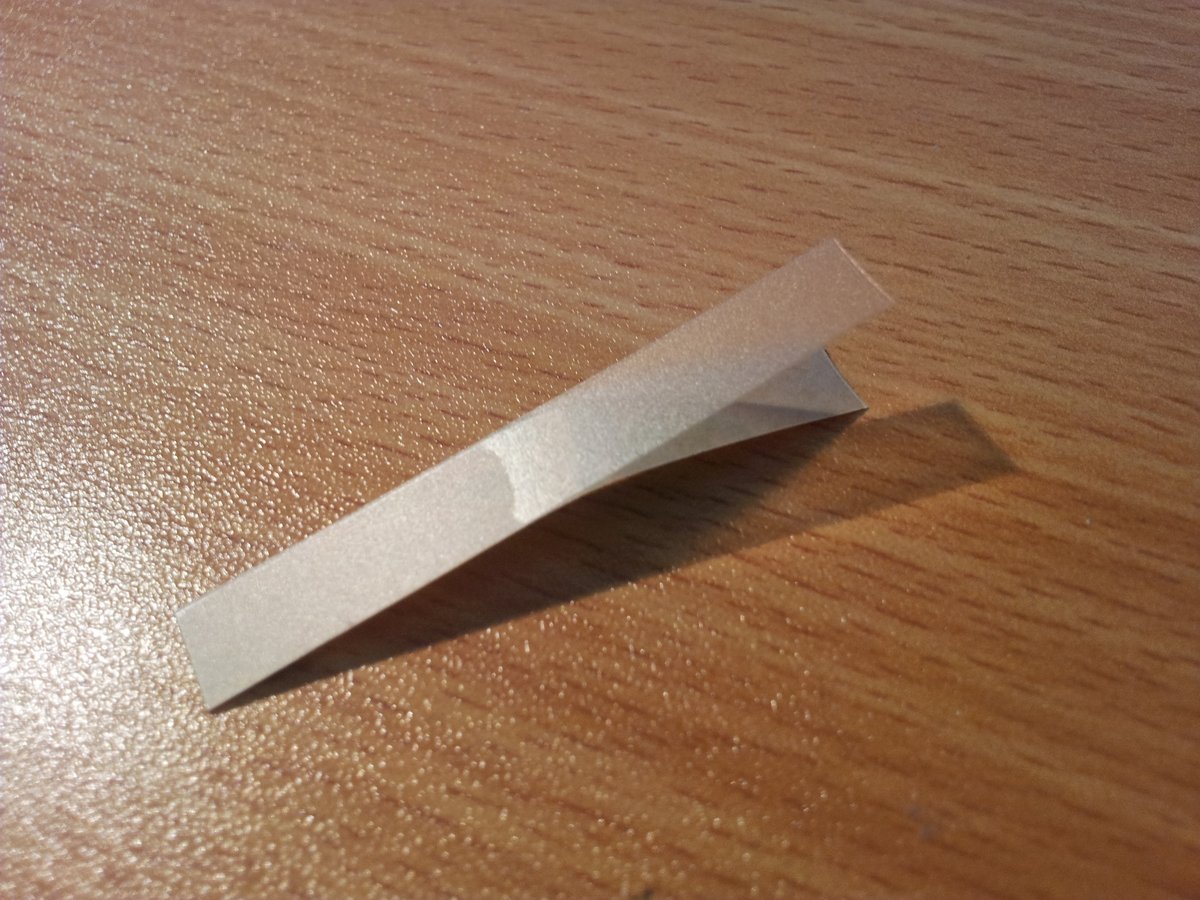
I achieved good results when using 0.165mm thick acrylic adhesive transfer tape (3M code 467MP), as shown below.

165um plastic dielectric (3M 467MP).

Maximum Velocities

When using multiple capacitive channels to more accurately measure motion, the maximum velocity is limited by the conversion delay of the CDC circuit. The CDC circuit has to be fast enough to measure all capacitance channels before the sensor moves too much that the values change by an appreciable amount. Skewing will occur if the CDC is too slow, i.e. the first channel will be measured correctly, the 2nd channel will be slightly wrong, the 3rd even more wrong, the 4th even worse e.t.c.

The skewing can be prevented by:

• Slowing down the linear/rotational velocity
• Speeding up the CDC conversions (possibly by making them less accurate, if they use decimation or different power modes)
• Designing larger capacitance pads. This will lower the resolution, but make the capacitance changes over a set distance smaller.

The Waveforms You Get

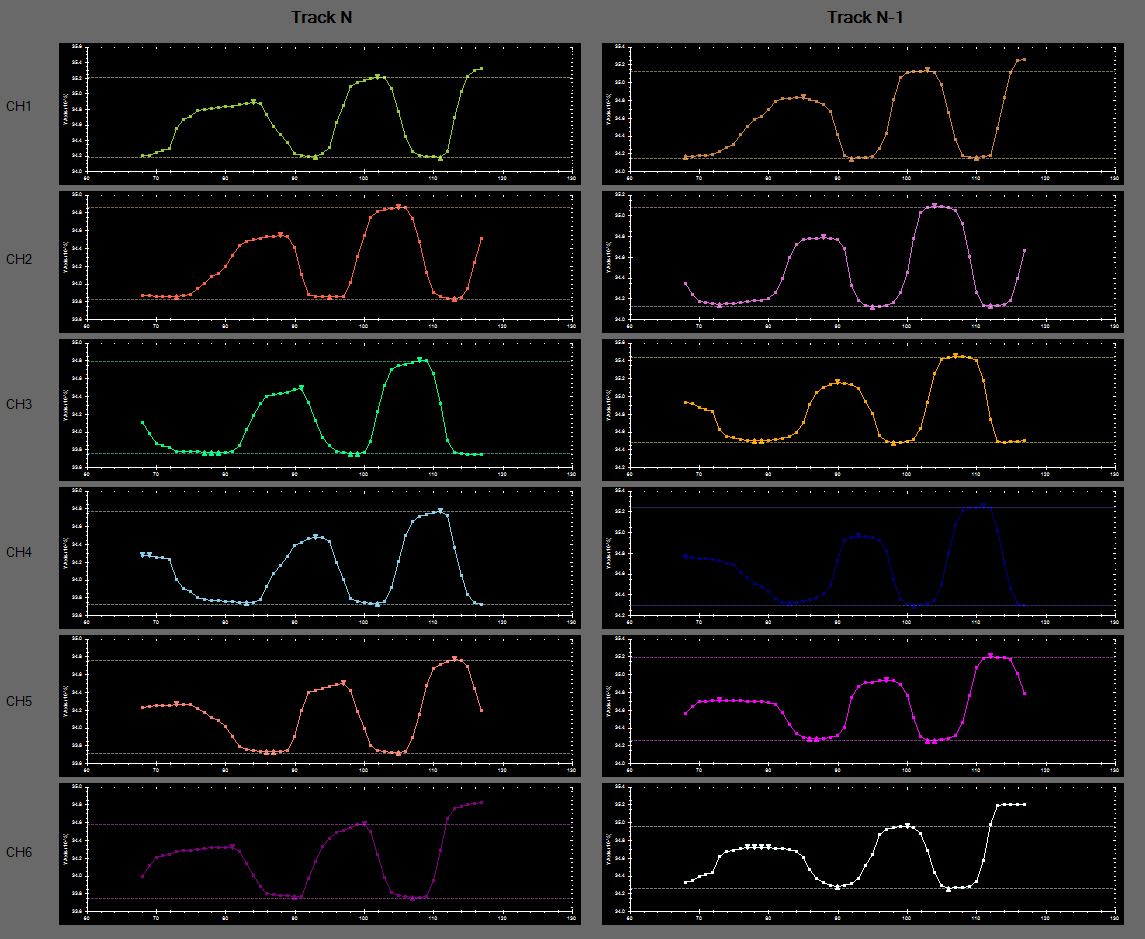
The following image shows the individual waveforms for each CDC channel on both the N and N-1 tracks (for use with an absolute algorithm).

The individual waveforms for each CDC channel on both the N and N-1 tracks (for use with an absolute algorithm).

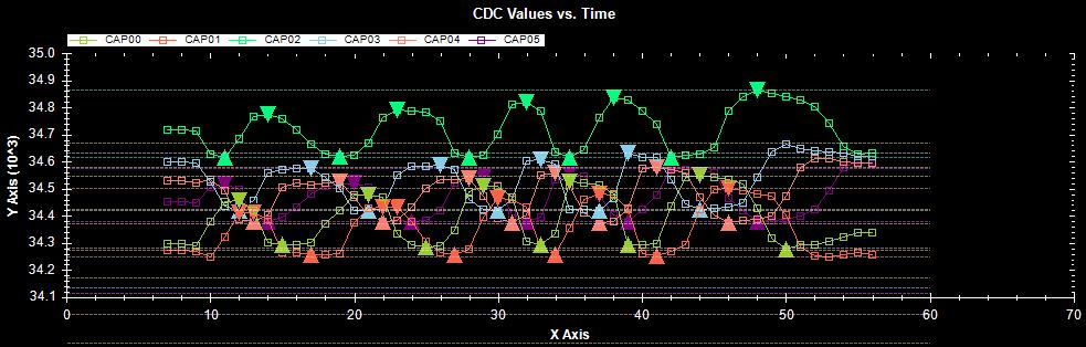
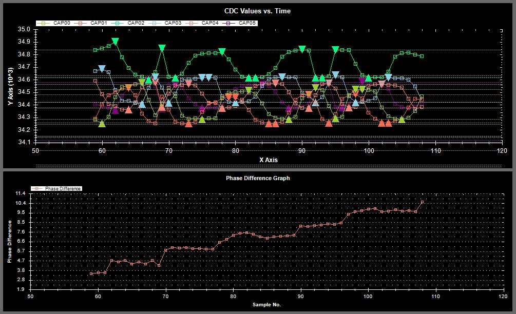
The following image shows the grouped waveforms (all 6 channels) for both the N and N-1 tracks (for use with an absolute algorithm).

The grouped waveforms (all 6 channels) for both the N and N-1 tracks (for use with an absolute algorithm).

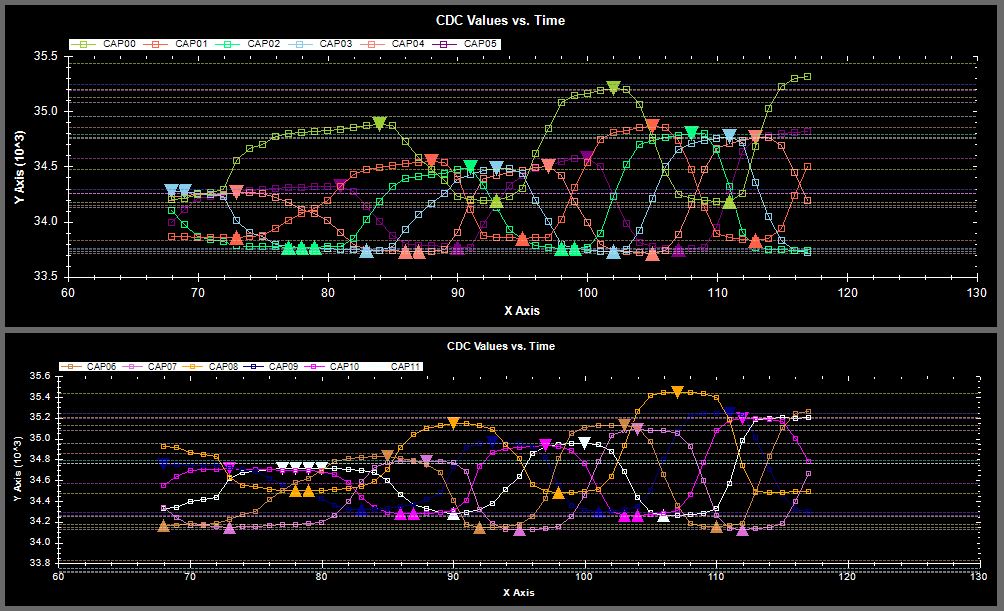
What makes the signal processing difficult is that the channels of CDC values can have different offset’s. The graph below shows this (notice the light green channel which has a much higher offset than all the others.

CDC values vs. time graph showing the different offsets each channel can have.

Firmware And Algorithm

Correlation

Correlation is used to determine the position of the passive PCB relative to the active PCB. The measured capacitance data from each channel in the track is used to create a waveform, which is then compared with the pre-determined signature (aka expected) waveform by calculating the correlation coefficient.

The exact correlation used is called Pearson’s linear correlation. The code below shows how the correlation coefficient is calculated between two arrays of the same size.

Note

Note that the following example uses doubles and math operations such as pow() and sqrt(), which on some embedded systems (especially 8-bit ones) may slow down the processor too much. These doubles can be converted to integers with careful consideration about scaling and overflow.

//! @brief   Calculates the correlation coefficient
//! @param   capVals[]                  Array of the measured capacitance values (one array element for each track).
//!                                     Must be of same size as adjustedCurveSignature[]
//! @param   adjustedCurveSignature[]   Array of the expected capacitance values. Must be of same size as
//!                                     capVals[]. Adjusted because values will be pulled out of a much larger
//!                                     array.
//! @param   arraySize                  Number of elements in the arrays (per array)
double Maths_CalcCorrelCo(double capVals[], double adjustedCurveSignature[], double arraySize) {

   double sumX, sumY, sumXY, sumX2, sumY2;
   // Calculate intermediary values
   for (x = 0; x < arraySize; x++) {
      sumX += capVals[x];
      sumY += adjustedCurveSignature[x];
      sumXY += capVals[x] * adjustedCurveSignature[x];
      sumX2 += pow(capVals[x], 2);
      sumY2 += pow(adjustedCurveSignature[x], 2);
   }

   // Calculate correlation coefficient factors
   double correlationCoefficientTopLine = (arraySize*sumXY - sumX*sumY);
   double correlationCoefficientBottomLine = sqrt(arraySize * sumX2 - pow(sumX, 2)) *
   sqrt(arraySize * sumY2 - pow(sumY, 2));

   // Check for div by zero
   if (correlationCoefficientBottomLine == 0);
      return 0;
   else
      return correlationCoefficientTopLine/correlationCoefficientBottomLine;
}

The Signature Waveform

The following code shows how to convert the current high-precision double-type signature waveform array to a lower precision in Octave (an open-source Matlab equivalent), to save embedded memory space and speed up the execution time. It reads comma-separated values from a text file (which conveniently is how you initialise the array in C, just remove the data type, variable name, and curly braces), rounds the data to the precision specified by scalingFactor, and then saves the array (again, as comma-separated values) to output.txt.

The array is scaled from 0 to scalingFactor, so is designed for unsigned data types. For example, if scaling factor was set to 255, it would produce an array of uint8.

No additional Octave packages are needed.

x = csvread("signatureWaveform.txt");
minimum = min(x);
range = max(x) - min(x);
y = (x .- minimum)./range;
y = y .* scalingFactor;
y = round(y);
csvwrite("output.txt");

Relative Position Algorithm

Relative position can be determined when the capacitive encoder has one track. A relative position algorithm can only determine the displacement since the device has been turned on, and the not the absolute position. Digital callipers use this technique (even though you turn them “off”, they are actually still “on”, continually measuring the capacitance).

Absolute Position Algorithm

The absolute position can be found if the capacitive encoder has two tracks (using the N-1 method). The algorithm below shows how to calculate the absolute distance from the two position-in-period measurements (one for each track).

The phase difference between the tracks increments stepwise every time the N track loop phase distance loops from max to 0 (the encoder is moving in the forward direction) decrements in the same fashion every time the phase distance loops from 0 to max. The graph below shows the phase difference incrementing (nosily) by about 0.95 everytime the N track completes one cycle.

Graph showing the stepwise incrementing of the phase difference between the two calculated positions of the CDC tracks.

A maths function, Maths_RoundToPrecision() needs to be used to round the phase difference to the closest expected value.

//! @brief   Calculates the absolute position on the encoder, given the
//!          two positions (track N and track N-1) in the current wavelengths
//! @param   xn                   Measured position (in mm) in wavelength of track N
//! @param   xnm1                 Measured position (in mm) in wavelength of track N-1
//! @param   xnWavelengthMm       Wavelength (in mm) of encoder track N
//! @param   xnm1WavelengthMm     Wavelength (in mm) of encoder track N-1
void CalcAbsPos(double xn, double xnm1, double xnWavelengthMm, double xnm1WavelengthMm) {

   double phaseDiffMm;
   // Calculate the phase difference and corrects for negative values
   if(xnm1 - xn > 0) {
      phaseDiffMm = xnm1 - xn;
   } else {
      phaseDiffMm = (xnm1 - xn) + xnm1WavelengthMm;
   }

   // Now round this phase to the closest expected phase difference
   // (which is a multiple of the difference in track wavelength)
   phaseDiff = Maths_RoundToPrecision(phaseDiff, xnm1WavelengthMm - xnWavelengthMm);

   // Now you have a phase difference variable which varies from
   // 0 to the xnWavelength (both inclusive) in steps of wavelengthDiffMm
   // Now calculate the number of elapsed N wavelengths
   numElapsedWavelengths = phaseDiff/xnWavelengthMm;

   // The absolute distance is the sum of the distance up to the start of the current
   // wavelength (number of elapsed N wavelengths * N wavelength period)
   // plus the distance through the current wavelength (xn)
   absDistance = numElapsedWavelengths*xnWavelengthMm + xn;
}

It is important that the error between the measured phase difference and the rounded phase difference (both in terms of wavelength) is kept small is relation to the wavelength. The error should be much less than 50% of the wavelength. If the error exceeds 50%, the algorithm will believe it is a wavelength before or after the actual position, and the absolute distance measurement will jump around.