Signal Processing

Child Pages

Overview

The Signal Processing section of this site covers digital filters (see Electronics->Circuit Design->Analogue Filters for the analogue counterpart), curve fitting, correlation, and signal feature detection.

The Math.Net project contains the “Neodym” library for signal processing in C#. The project can be downloaded, compiled in C# Express to produce a .dll, and then included as a resource in your own c# projects so you can then use the functions. I had issues using the DLL, and was getting the error “Could not load file: Strong name validation failed”.

To fix this, I needed to use sn.exe (a tool provided with Visual Studio and the Windows SDK, download either to use it), and to use the follow commands to skip strong name validation.

1

C:\project\mathnet-neodym\build\Debug>sn.exe -Vr *

Source Code

The opensource Math.Net NeoDym library contains C# code for using IIR filters.

Local Maxima/Minima (aka Peak/Trough) Detection

Maxima/minima detection is useful for frequency/phase detection of waveforms which have changing amplitude, DC bias, and frequency (i.e. are all over the place).

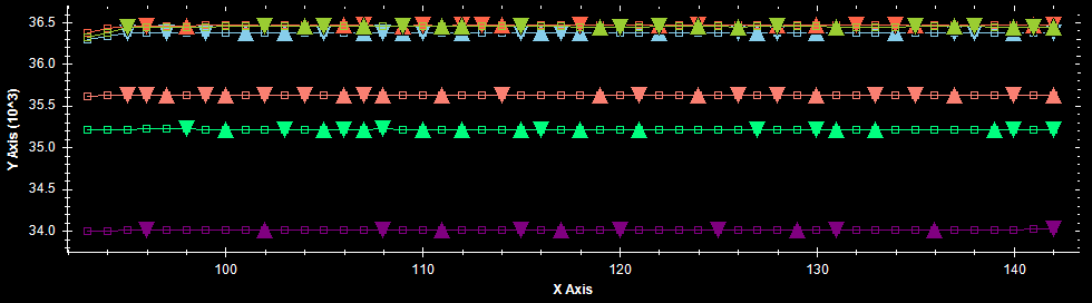
The following image shows maxima/minima detection for six noisy, sine-like waveforms.

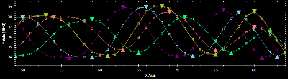
A graph on noisy, but stable data showing problems with maxima and minima detection without thresholding (false detections).

Iterating Over The Data

Unlike global maxima/minima (the largest and smallest values for a set of data), local maxima/minima detection is, however loosely, an online algorithm. You can process data to determine maxima/minima as the data is given to you. I mention the word loosely, because you have to have some previous and future data points, depending on the sampling window size.

Sampling Window

You need to specify a sampling window in which you are going to look for a local maximum/minimum in. This needs to be small enough so that multiple maxima or minima are not included in the window at the same time. The Hence the window size needs to be less than one period. The most basic window is a symmetric window (i.e. looking at the same number to data points to the left and right of the current index). The smallest symmetric window you could use would be 3 values wide. You need one value each side to make sure they are both lower (for a local maxima), or both higher (for a local minima).

However, real world data is not perfect, and is likely to have noise. This will cause false detections if only using a sample window of 3. Increasing this window size will decrease the number of false triggers due to noise. However, it won’t get rid of them, to do this, you also need thresholding (see below).

Local Extrema Code Libraries

I have written a C library, LocalExtrema, capable of finding local maxima/minima and designed to be run on embedded systems. It is hosted on GitHub here.

Correlation

Correlation is the measure of “likeness” between sets of data. The correlation coefficient tells you how well the two sets of data match. The Pearson’s correlation coefficient is given by:

wher`e:
\( X_i \) = value in data set one which is paired with
\( Y_i \) = value in data set two
\( \bar{X} \) = average value of data set 1
\( \bar{Y} \) = average value of data set 2

Detecting Variable Wraparounds

This is about how to detect if a variable which loops has “wrapped around”, that is, incremented from it’s highest value back to it’s lowest (a forward direction wraparound), or decremented from it’s lowest value back to it’s highest (a reverse direction wraparound).

Wraparounds (which are called overflows if they are not meant to happen in normal circumstances) occur in many digital signal processing situations. If you have a discrete, sampled variable which could potentially overflow, you cannot determine with 100% confidence whether an overflow occured.

For example, say you were measuring a signal which could take on a value between 1 and 10. Your first measurement returned the number 8, and the next measurement returned the number 1. Did the number overflow and jump forward 3 counts, or did it just jump backwards 7 counts?

The best you can do is make a statistical guess at which is more likely. In most real-world situations this would mean choosing the result which has the least absolute distance change, which in the example above would be deciding that it must of overflowed and jumped forward by 3 counts rather than jumping backwards by 7 counts.

Curve Fitting

Curve fitting is an essential part of signal processing.

Splines

A spline is a sufficiently smooth, piece-wise polynomial function. It is commonly used to fit a curve to a set of data. You also see them in vector-based drawing packages and 3D CAD programs.

Splines are most commonly a piece-wise collection of polynomials of degree \(n\), in where the first \(n - 1\) derivatives are equal at the points where the polynomials meet (remember it is piece-wise).

The most common type of spline is a cubic spline (a spline of order 3). The two most popular cubic splines are the cubic B-spline and cubic Bezier spline.

Splines have the advantage over a single polynomial in the fact the interpolation error can be lower for a given order (or for the same maximum interpolation error the order can be lower), which is less intensive computationally. Also, splines do no suffer from large edge-case errors as a single higher-degree polynomial would (Runge’s phenomenon).