Fourier Transforms

Overview

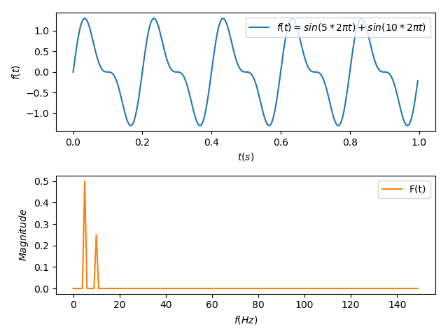
The Fourier transform is an operation which can transform a signal that is described in the time-domain (i.e. x-axis is time), into a signal that is described in the frequency-domain (the x-axis is frequency).

Fourier theorem states that a periodic function f(x) which is reasonably continuous may be expressed as the sum of a series of sine or cosine terms (called the Fourier series), each of which has specific amplitude and phase coefficients known as Fourier coefficients.¹

The finite signal in time has a continuous signal in frequency, and vice versa, a continuous signal in time has a finite signal in frequency.

The Fourier transform can be thought of as a rotation of 90 around the time-frequency domain. In this sense, four applications of the Fourier transform should result in the original signal.

There are four common Fourier transformations, which are described below:

Continuous-Time Fourier Transform (CTFT)

The Continuous-Time Fourier Transform (CTFT) is also commonly known just as the Fourier Transform. There is a definition of the equation which converts a signal in time to a signal in frequency, which is called the forward transform, and one which goes from the frequency domain back to the time domain (it undoes the forward transform) called the inverse transform.

Note that the variable \(t\) (the independent variable) does no have to necessarily represent time. However, when it does (e.g. units in seconds), then the transform variable \(f\) represents frequency (e.g. Hertz). All of the equations below will use t and f since time and frequency are the most common units used with the Fourier transform.

Forward:

$$ F(f) = \int_{-\infty}^{\infty} f(t) e^{-j2\pi ft} dt $$

Inverse:

$$ f(t) = \int_{-\infty}^{\infty} F(f)e^{i2\pi ft} df $$

Continuous-Time Fourier Series (CTFS)

Forward:

$$ F_n = \frac{1}{T_0} \int_{-\frac{T_0}{2}}^{\frac{T_0}{2}} f(t) e^{\frac{-j2\pi nt}{T_0}}dt $$

Inverse:

$$ x(t) = \sum_{n=-\infty}^{\infty} F_n e^{\frac{j 2\pi nt}{T_0}} $$

Discrete-time Fourier Transform (DTFT)

The DTFT of a discrete time serious produces a frequency signal that is continuous and periodic.

Forward:

$$ F(e^{j\omega}) = \sum_{n=-\infty}^{\infty} f(nT)e^{-j2\pi fnT} $$

Inverse:

$$ f(nT) = \int_{-\frac{1}{2T}}^{\frac{1}{2T}} F(e^{j\omega})e^{j2\pi fnT} df $$

Discrete Fourier Transform (DFT)

Forward:

$$ F(\frac{k}{NT}) = \sum_{n=0}^{N-1} f(nT)e^{\frac{-j2\pi nk}{N}} $$

Inverse:

$$ f(nT) = \frac{1}{N} \sum_{k=0}^{N-1}F\frac{k}{NT}e^{\frac{i2\pi nk}{N}} $$

The Fast Fourier Transform (FFT)

A fast fourier transform is a way of calculating the DFT (discrete fourier transform) of a signal. A fourier transform is a way of looking at a waveform in the time domain to see what frequencies it is made up of. A fast fourier transform differentiates itself apart from a standard fourier transform by factorizing the DFT matrix into a produce of sparse (mostly zero) factors. This actions reduces the complexity of the DFT algorithm from \( \mathcal{O}(n^2) \) to \( \mathcal{O}(n\log{n}) \). This speed increase means that the FFT is very popular in signal processing applications.

Bin Size

The width of each bin (in Hertz) is equal to:

where:
\( f_s \) is the sample rate, in Hertz
\( N_{bins} \) is the number of bins

The bins of interest are those from \( 0 \) to \( \frac{N_{bins}}{2} \).

Sampling Rate

By the Nyquist-Shannon sampling theorem, if the sampling rate is say, 10kHz, then the maximum captured frequency content will be 5kHz. This is true when using FFTs.

However, sampling just at the Nyquist rate does not give you great data. As a rule-of-thumb, if you want to accurately find the frequencies present in a signal with a reasonably low number of samples, the sample rate should be about 10x the maximum frequency of interest.

Number of Samples

FFT algorithms require a number of samples which is equal to an integer power of two (e.g. 2, 4, 8, 16, …).

Frequency vs. Temporal Resolution

There is always a trade-off between frequency and temporal (time based) resolution. At a fixed sample rate, increasing the frequency resolution decreases the temporal resolution. To increase the frequency resolution, you have to increase the number of bins. This will make a single FFT window take longer to run, which decreases the temporal resolution (all temporal info within a single FFT window is lost).

Windowing

A FFT samples a waveform to a finite length (you don’t/can’t measure the signal for time negative infinity to positive infinity) in what is called the window. An FFT algorithm also assumes the signal within the window repeats forever. With most real-world signals, this will result in discontinuities at the edges of the window (the only time this does not happen is if the signal repeats itself, and the window happens to contain an exact integer number of cycles).

If nothing is done to the edges of the window, you will get significant spectral leakage. One way to reduce the spectral leakage is to perform windowing, in where the signal is faded in and out in the first few/last few samples.

The 2D Fourier Transform And Images

Because most images are stored digitally, the Discrete Fourier Transform (DFT) is used.

Taking an standard input image which is in the spatial domain, the 2D DFT converts the image into the frequency domain. Each pixel in the output image represents a particular frequency in the input spatial domain image.

The number of frequencies in the image is equal to the number of pixels in the image. Obviously, this means that the frequency domain image will the same size as the spatial domain image.

The definition of the 2D Fourier transform (continuous):

$$ \mathcal{F}(u,v) = \int_{-\infty}^{\infty} \int_{-\infty}^{\infty} f(x,y) e^{-j2\pi(ux + vy)} dx\,dy $$

Converted into a 2D discrete Fourier transform, the equation becomes:

$$ \mathcal{F}(k, l) = \sum_{i=0}^{N-1} \sum_{i=0}^{N-1} f(i,j) e^{-i2\pi (\frac{ki}{M} + \frac{lj}{N})} $$

where:
\( f(i, j) \) is the image in the spatial domain

The basis functions are sine and cosine waves with increasing frequencies. \(\mathcal{F}(0, 0)\) represents the DC component in the image (the average brightness), all the way up to \(\mathcal{F}(N-1, N-1)\) which represents the highest frequency in the image. Note that \(\mathcal{F}(0, 0)\) is usually shifted to be in the center of the frequency domain image.

The Fourier Transform of a real-numbered spatial image (i.e. a typical photo) produces a complex-valued image in the frequency domain. Obviously, we can’t view an image made of complex numbers. What we can do is display the frequency domain image as two images, either:

• 1 image contains the real part of the complex number, the other image displays the imaginary part
• 1 image displays the magnitude, the other image displays the phase (the argument of the complex number)

Often in image processing, we use the magnitude/phase representation, and are mostly interested in the magnitude image. The magnitude can be written as \(|F(u,v)|\), the phase as \(\phi F(u,v) \)

Code Libraries

The opensource Math.Net Numerics library contains C# FFT code built for the .NET framework.

External Resources

The Fourier Transform series on The Mobile Studio must be one of the best online resources if you are looking into learning more about the Fourier Transform. It is a very detailed yet well explained step-by-step tutorial!