Algorithm Time Complexity

Algorithmic time complexity is a measure of how long it takes for an algorithm to complete when there is a change in size of the input to the algorithm (which is usually the number of elements, $n$. Rather than actually measure the time taken, which varies on the programming language, processor speed, architecture, and a hundred other things, we consider the “time” to be the number of basic operations that the algorithm has to take. This gives us an metric independent on the users computer, that we can use to rate one algorithm against another when solving a problem.

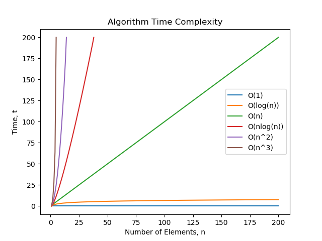
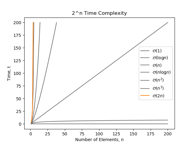
A graph showing the response of different time complexities as the number of elements increase. Coefficients were chosen so that the worst time complexities were the largest by the time n = 1000.

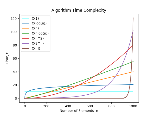
A graph showing the response of different time complexities as the number of elements increase. Coefficients were chosen so that the worst time complexities were the largest by the time n = 1000.

Big-O, Little-o, Theta And Omega

Big-O (pronounced “Big-Oh”), little-o, Theta and Omega are all mathematical methods of describing an algorithms growth as the size of the input increases. We can look at growth in two different ways: the increase in computational cost and the increase in storage (memory).

There are three different mathematical notations used:

• $\mathcal{O}(f(n))$ (Big-O) describes the upper bound in complexity
• $\mathcal{o}(f(n))$ (little-O) also describes the upper bound in complexity, but is a stronger statement. Big-O is in inclusive upper bound (grows less than or equal to), while little-o is a strict upper bound (grows strictly less than). Big-O is to little-o as $\leq$ is to $\le$.
• $\Omega(f(n))$ describes the lower bound in complexity
• $\Theta(f(n))$ describes the exact bound in complexity

$\mathcal{O}(f(n))$ (Big-O) is the most commonly used complexity, as we are normally interested in the worst case computational cost/memory usage when choosing/designing an algorithm. Note that you even when using Big-O, you can still talk about average-case and worst-case scenarios, but this is referring to specific inputs and algorithms states which cause the algorithm to perform more poorly than usual.

Normally, we use Big-O notation to describe time complexity (computational cost). Basically, it’s a big $\mathcal{O}()$ with brackets, and inside the bracket you write how the time complexity scales with the input. The input is usually called $n$, and usually represents the “number of things/elements/objects” the algorithm has to deal with.

Big-O notation ignores and constant terms and any constant coefficients (e.g. an algorithm that grows at $2n$ is still written as $\mathcal{O}(n)$. This is because constant terms and constant coefficients do not effect the growth, you can think as Big-O notation as kind of analysis on the “derivative”.

Complexity Algebra

When adding two big-O complexity classes we can move the functions inside the $\mathcal{O}$:

$\mathcal{O}(f(n)) + \mathcal{O}(g(n)) = \mathcal{O}(f(n) + \mathcal{O}(g(n)))$

Then the larger complexity class becomes dominant and we drop the lower class. For example:

$\mathcal{O}(n) + \mathcal{O}(log(n)) = \mathcal{O}(n + log(n)) = \mathcal{O}(n)$

$n$ grows faster than $\log{n}$, as $\lim_{n \to \infty} \frac{\log{n}}{n} = 0$.

Common Complexity Classes

The following complexity classes are described from best to worst.

Note

All Big-O complexities examples below are assumed to be average-case, unless specified otherwise.

Constant Time

The growth of constant time complexity compared with other common complexity classes.

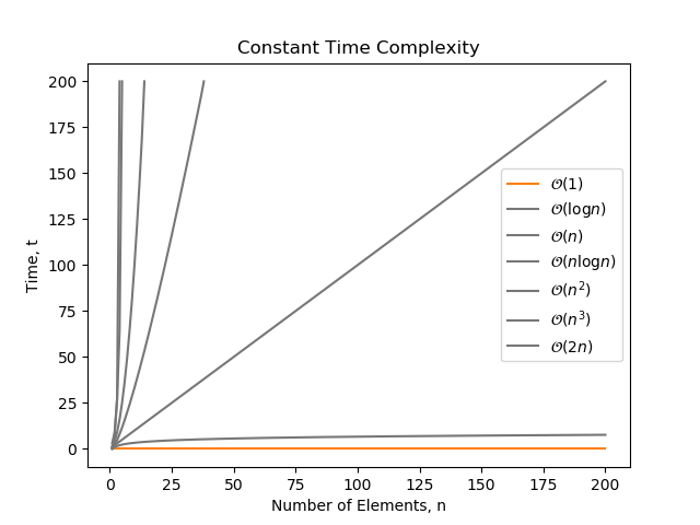
The following algorithm just prints “hello” once, and doesn’t depend on the number of elements ($n$). It will always run in constant time, and therefore is $\mathcal{\mathcal{O}}(1)$.

print('hello')

Note that even though the following algorithm prints out hello three times, it still does not depends on $n$, and runs in constant time. Again, it is still classified as $\mathcal{O}(1)$.

print('hello')
print('hello')
print('hello')

$\mathcal{O}(1)$ complexity is the best algorithm complexity you can achieve. Common software operations that have $\mathcal{O}(1)$ complexity are:

• Reading a value from an array (e.g. a Python list, a C array, or a C++ std::vector). To read a value from a from an array, you just read the memory address at base_address + index * value_size. This takes a constant amount of time, no matter the size of the array.
• Reading an element from hash table (e.g. a Python dictionary). Computing the hash of a key takes a constant amount of time, and then looking up the memory location at that hash is also constant.
• Deleting an element from a doubly-linked list.
• Push/pop of a stack.
• Inserting a value at the end of an array (note, this is amortized $\mathcal{O}(1)$ complexity)

Note

Even if an algorithm takes a long time to calculate something, e.g. computing a hash, as long as this operation takes the same amount of time, no matter if there are 3 elements or 9000, it is still considered $\mathcal{O}(1)$.

log(n) Time

The growth of logarithmic time complexity compared with other common complexity classes.

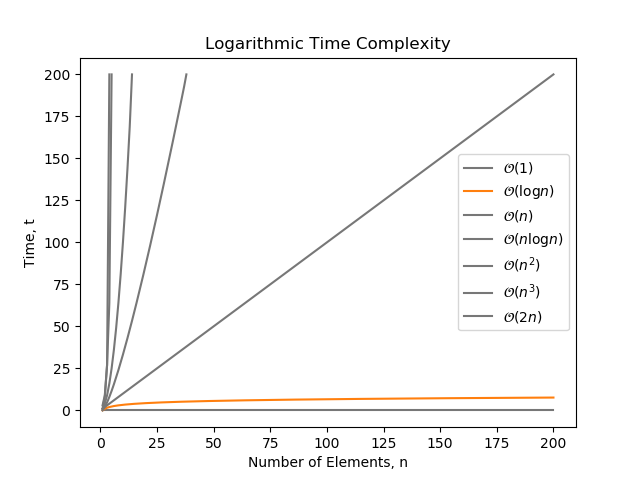
$\mathcal{O}(\log{n})$ is a time complexity where the number of operations grows with the logarithm of the size of the input. $\mathcal{O}(\log{n})$ complexity is considered to be pretty good. You can think of it as: Every time the size of the input doubles, the complexity increases by a constant amount.

Note that whenever we are talking about software algorithms with $\mathcal{O}(\log{n})$ complexity, we are usually referring $\mathcal{O}(\log_2{n})$ complexity (due to the binary nature of most algorithms). However, this does not matter, as all logarithmic complexities belong to the same class, no matter what the base is. The base is just a constant factor which again disappears (e.g. $\frac{\log{1000}}{\log{10}} = 2$, no matter what base is used).

i = 0
while i < n:
    print('hello')
    i *= 2 # Double i each time, making it O(log n)

Notice the i *= 2, which makes in run in $\mathcal{O}(\log{n})$ time.

Common software operations that have $\mathcal{O}(\log{n})$ complexity are:

• Finding an element in a binary search tree. a 1-node binary tree has height $\log_2{1} + 1 = 1$, a 2-node binary tree has height $\log_2{2} + 1 = 2$, a 4-node binary tree has height $\log_2{4} + 1 = 3$, and so on. An n-node tree has height $\log_2{n} + 1$, so adding elements to the tree causes the height to grow logarithmically with the number of inputs.
• A binary search algorithm. On each iteration you half the number of elements remaining in the search space.
• The best way to calculate Fibonacci numbers (the easiest way with recursion is $\mathcal{O}(2^n)$!).
• Calculating $a^n$.
• Other “divide-and-conquer” style algorithms.

Linear Time

The growth of linear time complexity compared with other common complexity classes.

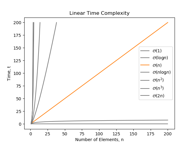
Linear time is when an algorithm grows at a rate proportional to the number of elements, $n$. A simple for loop has $\mathcal{O}(n)$ complexity:

for i in range(n):
    print('hello')

Another example:

for i in range(0, n, 2): # Increment n by 2 each time
    print('hello')

Note that even though the above example prints “hello” for every second $n$ (so it performs $0.5n$ prints), it still has $\mathcal{O}(n)$ complexity (remember that coefficients are dropped).

nlog(n) Time

The growth of nlogn time complexity compared with other common complexity classes.

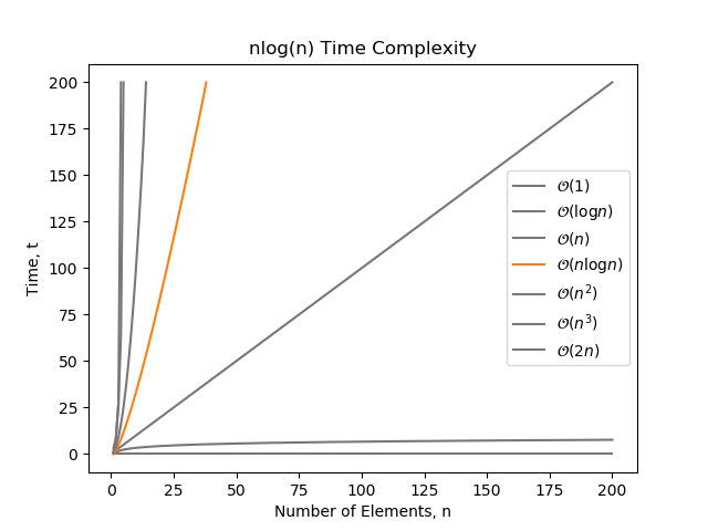
$\mathcal{O}(n\log{n})$ complexity can be thought of as a combination of $\mathcal{O}(n)$ and $\mathcal{O}(\log{n})$ complexity (and more often than not, this is how the algorithm actually works). It is famously known as the best complexity that you can sort an arbitrary collection of elements in.

This can be demonstrated by a nested for loop, one having $\mathcal{O}(n)$ complexity and the other $\mathcal{O}(\log{n})$ complexity:

for i in range(n):
    j = 0
    while j < n:
        print('hello')
        j *= 2 # This inner loop is log(n)

Examples of $\mathcal{O}(n\log{n})$ complexity:

• Merge sort
• Heap sort
• Quick sort

n^2 Time

The growth of n^2 time complexity compared with other common complexity classes.

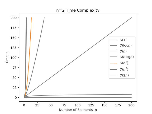
$\mathcal{O}(n^2)$ complexity is proportional to the square of the number of elements $n$. This is a bad form of complexity to have, especially when $n$ grows large.

The most basic example of $\mathcal{O}(n^2)$ is a pair of nested for loops, each iterating over every element:

for i in range(n):
    for j in range(n):
        print('hello')

Here is another example which has $\mathcal{O}(n^2)$ complexity:

for i in range(n):
    for j in range(n):
        print('hello')

for i in range(n):
    for j in range(n):
        print('hello')

Note that this is just a 2x repetition of a algorithm with $\mathcal{O}(n^2)$ complexity. Repeating an algorithm (i.e. performing it twice) does not change the complexity.

n^3 Time

The growth of n^3 time complexity compared with other common complexity classes.

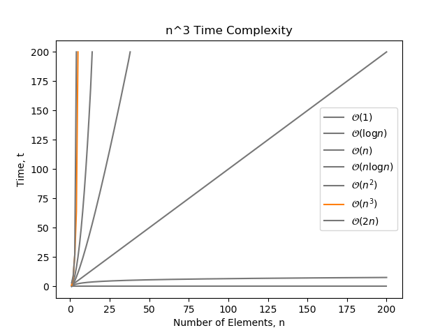
$\mathcal{O}(n^3)$ complexity is rarely seen in a single software algorithms (but can easily arise from the combination of multiple algorithms to solve a problem).

for i in range(n):
    for j in range(n):
        for k in range(n):
            print('hello')

Naturally, we could keep going forever explaining poorer and poorer complexities ($n^4$, $n^5$, e.t.c), but I think by now you understand the concept, and these higher complexities are rarely seen in real software algorithms.

2^n Time

The growth of 2^n time complexity compared with other common complexity classes.

Exponential time is written as $\mathcal{O}(2^n)$. Exponential time is always greater than any polynomial time, e.g. $2^n$ grows faster than $n^{1000}$.

An example of $\mathcal{O}(2^n)$ time is the naive (and simple) implementation of an algorithm that calculates the Fibonacci sequence, without the use of dynamic programming. It would look something like this:

def fibonacci(n):
    if n <= 1:
        return n
    else
        return fibonacci(n - 1) + fibonacci(n - 2)

n! Time

Factorial time is written as $\mathcal{O}(n!)$. It is a very rare and hugely expensive complexity class. Permutation algorithms.

Exotic Times

• The infamous Bogo sort runs in $\mathcal{O}(n \cdot n!)$ time.

Amortized Complexity

When we talk about amortized complexity, we are referring to complexity per run, as the number of runs goes to infinity. This means that if sometimes, the runtime is much longer, as long as this event is infrequent enough, the amortized complexity can still be quite good.

In formal terms:

Amortized complexity is the total expense per operation, evaluated over a sequence of operations.

For example, take the example of adding a value to an array. The array starts of being able to hold one value, and it’s size is doubled every time we run out of space. When we add a value, it normally doesn’t need resizing, which is $\mathcal{O}(1)$. But when adding the 1st, 2nd, 4th, 8th, 16th, e.t.c value, we need to resize the array. This takes $\mathcal{O}(n)$. The probability of having to resize the array is $\frac{1}{n}$. This gives an amortized complexity of $\frac{\mathcal{O}(n)}{n} = \mathcal{O}(1)$.

Amortized complexity is not the same thing as average complexity.