Polynomial Curve Fitting

Overview

Before reading this page, please check out the Linear Curve Fitting page. Many of the principles mentioned there will be re-used here, and will not be explained in as much detail.

Calculating The Polynomial Curve

We can write an equation for the error as follows:

$$\begin{align} err & = \sum d_i^2 \nonumber \\ & = (y_1 - f(x_1))^2 + (y_2 - f(x_2))^2 + (y_3 - f(x_3))^2 \nonumber \\ & = \sum_{i = 1}^{n} (y_i - f(x_i))^2 \end{align}$$

where:
\(n\) is the number of points of data (each data point is an \(x, y\) pair)
\(f(x)\) is the function which describes our polynomial curve of best fit

Since we want to fit a polynomial, we can write \(f(x)\) as:

$$\begin{align} f(x) &= a_0 + a_1 x + a_2 x^2 + ... + a_n x^n \nonumber \\ &= a_0 + \sum_{j=1}^k a_j x^j \end{align}$$

where:
\(k\) is the order of the polynomial

Substituting into above:

$$\begin{align} err = \sum_{i = 1}^{n} (y_i - (a_0 + \sum_{j=0}^k a_j x^j))^2 \end{align}$$

How do we find the minimum of this error function? We use the derivative. If we can differentiate \(err\), we have an equation for the slope. We know that the slope will be 0 when the error is at a minimum.

We have \(k\) unknowns, \(a_0, a_1, ..., a_k \). We have to take the derivative of each unknown separately:

$$\begin{align} \frac{\partial err}{\partial a_0} &= -2 \sum_{i=1}^{n} (y_i - (a_0 + \sum_{j=0}^k a_j x_j)) &= 0 \nonumber \\ \frac{\partial err}{\partial a_1} &= -2 \sum_{i=1}^{n} (y_i - (a_0 + \sum_{j=0}^k a_j x_j))x &= 0 \nonumber \\ \frac{\partial err}{\partial a_1} &= -2 \sum_{i=1}^{n} (y_i - (a_0 + \sum_{j=0}^k a_j x_j))x^2 &= 0 \nonumber \\ \vdots \nonumber \\ \frac{\partial err}{\partial a_k} &= -2 \sum_{i=1}^{n} (y_i - (a_0 + \sum_{j=0}^k a_j x_j))x^k &= 0 \\ \end{align}$$

These equations can be re-arranged into matrix form:

We solve this by re-arranging (which involves taking the inverse of \(\bf{x}\))`:

Thus a polynomial curve of best fit is:

See main.py for Python code which performs these calculations.

Worked Example

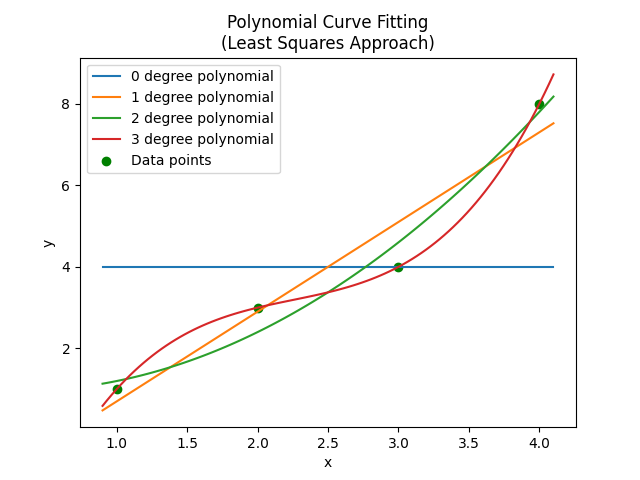
Find a 2 degree polynomial that best describes the following points:

We will then find the values for each one of the nine elements in the \(\mathbf{A}\) matrix:

$$\begin{align} A_{11} &= n = 4 \nonumber \\ A_{12} &= \sum x_i = 1 + 2 + 3 + 4 = 10 \nonumber \\ A_{13} &= \sum x_i^2 = 1^2 + 2^2 + 3^2 + 4^2 = 30 \nonumber \\ A_{21} &= A_{12} = 10 \nonumber \\ A_{22} &= A_{13} = 30 \nonumber \\ A_{23} &= \sum x_i^3 = 1^3 + 2^3 + 3^3 + 4^3 = 100 \nonumber \\ A_{31} &= A_{22} = 30 \nonumber \\ A_{32} &= A_{23} = 100 \nonumber \\ A_{33} &= \sum x_i^4 = 1^4 + 2^4 + 3^4 + 4^4 = 354 \\ \end{align}$$

And now find the elements of the \(\mathbf{B}\) matrix:

$$\begin{align} B_{11} &= \sum y_i = 1 + 3 + 4 + 8 = 16 \nonumber \\ B_{21} &= \sum x_i y_i = 1*1 + 2*3 + 3*4 + 4*8 = 51 \nonumber \\ B_{31} &= \sum x_i^2 y_i = 1^2*1 + 2^2*3 + 3^2*4 + 4^2*8 = 177 \nonumber \\ \end{align}$$

Plugging these values into the matrix equation:

We can then solve `\(\mathbf{x} = \mathbf{A^{-1}}\mathbf{B}\) by hand, or use a tool. I used Python’s NumPy package to end up with:

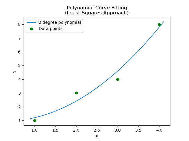
Thus our line of best fit:

The data points and polynomial of best fit are shown in the below graph: