Linear Curve Fitting

Fitting A Linear Curve (Line)

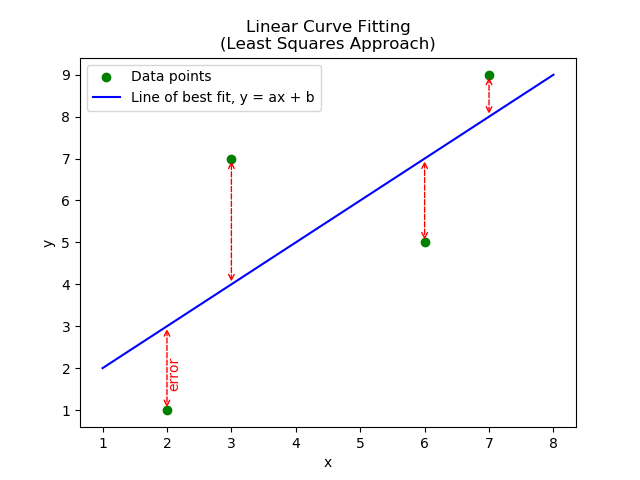
Fitting a linear curve (a line!) to a set of data is called linear regression. Typically, we want to minimize the square of the vertical error between each point and the line. The following graph shows four data points in green, and the calculated line of best fit in blue:

The linear curve fitting (using the least squares approach) to four data points.

We can write an equation for the error as follows:

$$\begin{align} err & = \sum d_i^2 \\ & = (y_1 - f(x_1))^2 + (y_2 - f(x_2))^2 + (y_3 - f(x_3))^2 \\ & = \sum_{i = 1}^{n} (y_i - f(x_i))^2 \end{align}$$

where:
$n$ is the number of points of data (each data point is an $x, y$ pair)
$f(x)$ is the function which describes our line of best fit

Since we want to fit a straight line, we can write $f(x)$ as:

$$f(x) = ax + b$$

Substituting into above:

$$err = \sum_{i = 1}^{n} (y_i - (ax_i + b))^2$$

How do we find the minimum of this error function? We use the derivative. If we can differentiate $err$, we have an equation for the slope. We know that the slope will be 0 when the error is at a minimum.

Because we are solving for two unknowns, $a$ and $b$, we have to take the derivative of both separately:

$$\frac{\partial err}{\partial a} = -2 \sum_{i=1}^{n} x_i(y_i - ax_i - b) = 0$$ $$\frac{\partial err}{\partial b} = -2 \sum_{i=1}^{n} (y_i - ax_i - b) = 0$$

We now have two equations and two unknowns, we can solve this! Lets re-write the equations in the form $C_1 a + C_2 b = C_3$:

$$\begin{align} & (\sum x_i^2) a & + (\sum x_i) b &= \sum x_i y_i \\ & (\sum x_i) a & + (n) b &= \sum y_i \end{align}$$

We will put this into matrix form so we can easily solve it:

$$\begin{bmatrix} \sum x_i^2 & \sum x_i \\ \sum x_i & n \end{bmatrix} \begin{bmatrix} a \\ b \end{bmatrix} = \begin{bmatrix} \sum x_i y_i \\ \sum y_i \end{bmatrix}$$

We solve this by re-arranging which involves taking the inverse of x):

$$\mathbf{x} = \mathbf{A^{-1}} \mathbf{B}$$

Thus a linear curve of best fit is:

$$y = x[0] x + x[1]$$

See https://github.com/gbmhunter/BlogAssets/tree/master/Mathematics/CurveFitting/linear for Python code which performs these calculations.

Worked Example

EXAMPLE: Find a line of best fit

Find the line of best fit for the following points:

$$(2, 1) \\ (3, 7) \\ (6, 5) \\ (7, 9)$$

We will then find the values for each one of the four elements in the $\mathbf{A}$ matrix:

$$\begin{align} A_{11} &= \sum x_i^2 = 2^2 + 3^2 + 6^2 + 7^2 = 98 \\ A_{12} &= \sum x_i = 2 + 3 + 6 + 7 = 18 \\ A_{21} &= \sum x_i = 2 + 3 + 6 + 7 = 18 \\ A_{22} &= n = 4 \end{align}$$

And now find the elements of the $\mathbf{B}$ matrix:

$$\begin{align} B_{11} &= \sum x_i y_i = 2*1 + 3*7 + 6*5 + 7*9 = 116\\ B_{21} &= \sum y_i = 1 + 7 + 5 + 9 = 22 \end{align}$$

Plugging these values into the matrix equation:

$$\begin{bmatrix} 98 & 18 \\ 18 & 4 \end{bmatrix} \begin{bmatrix} a \\ b \end{bmatrix} = \begin{bmatrix} 116 \\ 22 \end{bmatrix}$$

We can then solve $\mathbf{x} = \mathbf{A^{-1}}\mathbf{B}$ by hand, or use a tool. I used Python’s NumPy package to end up with:

$$\begin{bmatrix}a \\ b\end{bmatrix} = \begin{bmatrix}1 \\ 1\end{bmatrix}$$

Thus our line of best fit:

$$y = 1x + 1$$

The points and line of best fit are shown in the below graph:

The linear curve fitting (using the least squares approach) to four data points.